3DB: A Framework for Debugging Vision Models

    Paper    Project Repo    Documentation and Guides    Blog Demo

In our latest paper, in collaboration with Microsoft Research, we introduce 3DB: an extendable, unified framework for debugging and analyzing vision models using photorealistic simulation. We’re releasing 3DB as a package, accompanied by extensive API documentation, guides, and demos.

Note: this post contains some interactive plots and 3D models that use JavaScript: click here for a JS-free version of this post.

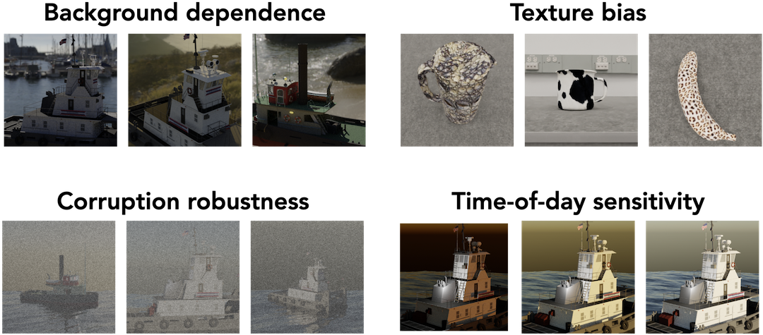
Identifying failure modes and biases in vision models is a rapidly emerging challenge in machine learning. In high-stakes applications, simply deploying models and collecting failures that arise in the wild is often difficult, expensive, and irresponsible. To this end, a recent line of work in vision focuses on identifying model failure modes via in-depth analyses of image transformations and corruptions, object orientations, backgrounds, or shape-texture conflicts. These studies (and other similarly important ones) reveal a variety of patterns of performance degradation in vision models. Still, performing each such study requires time, developing (often complex) toolingFor our study of image backgrounds, for example, we used a combination of bounding boxes and classical computer vision tools to crop out image backgrounds. We then had to manually filter out the images for which the tools failed. Even for the images where the toolkit succeeded, there remained inevitable cropping artifacts., and a willingness to settle for less than perfect simulations of each potential failure mode. Our question is: can we support reliable discovery of model failures in a systematic, automated, and unified way?

3DB: A Rendering-based Debugging Platform

In our latest paper, we try to make progress on this question and propose 3DB, a platform for automatically identifying and analyzing the failure modes of computer vision models using 3D rendering. 3DB aims to allow users to go from a testable, robustness-based hypothesis to concrete, photorealistic experimental evidence with minimal time and effort.

The platform revolves around the modular workflow pictured below. First, users specify a set of 3D objects and environments, as well as a set of 3D (or 2D) transformations called controls that determine the space of admissible object-environment configurations. 3DB then renders a myriad of admissible scenes and feeds them through the user’s computer vision model of choice. The user can finally stratify, aggregate, or otherwise analyze the results either by reading the outputted JSON, or through the pre-packaged dashboard.

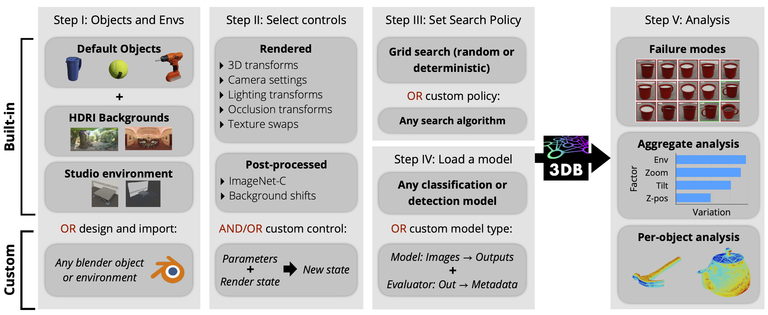
3DB easily adapts to a variety of use cases: in particular, users can modify and swap out any part of this pipeline (e.g., the renderer, the logger, the model type, or the controls) for their own custom-written components, without needing to modify any of the 3DB codebase. We’ve compiled guides, extensive API documentation, and a full demo showing how 3DB streamlines model debugging.

In fact, this blog post will double as another demo! We’ll present the (short) code necessary to reproduce every plot in the post below using 3DB. You can download the aggregated code for this blog post here.

To set up, follow the steps below—then, in the remainder of this post, press “Show/hide code and instructions” to see the steps necessary to reproduce each experiment below.

inference:
  module: 'torchvision.models'
  label_map: 'blog_demo/resources/imagenet_mapping.json'
  class: 'resnet18'
  normalization:
    mean: [0.485, 0.456, 0.406]
    std: [0.229, 0.224, 0.225]
  resolution: [224, 224]
  args:
    pretrained: True
evaluation:
  module: 'threedb.evaluators.classification'
  args:
    classmap_path: 'blog_demo/resources/ycb_to_IN.json'
    topk: 1
render_args:
  engine: 'threedb.rendering.render_blender'
  resolution: 256
  samples: 16
policy:
  module: "threedb.policies.random_search"
  samples: 5
logging:
  logger_modules:
    - "threedb.result_logging.image_logger"
    - "threedb.result_logging.json_logger"

Using 3DB

Prior works have already used 3D rendering (to great effect) to study biases of machine learning models, including pose and context-based biases. Our goal is not to propose a specific 3D-rendering based analysis, but rather to provide an easy-to-use, highly extendable framework that unifies prior analyses (both 3D and 2D) while enabling users to (a) conduct a host of new analyses with the same ease and with realistic results; and (b) effortlessly compose different factors of variation to understand their interplay.

We’ll dedicate the rest of this post to illustrating how one might actually use 3DB in practice, focusing on a single example 3D model3DB works with any 3D model, and we refer the reader to our paper for more examples and details.:

In what follows, we will walk through example applications of 3DB to discover biases of ML models (some previously documented, others not). For the sake of brevity, we’ll highlight just a few of these (re-)discoveries—to see more, check out the paper. We’ll then demonstrate that the discoveries of 3DB transfer pretty reliably to the real world!

Our experiments will all operate on an ImageNet-pretrained ResNet-18The classifier has a ~70% validation-set accuracy. that has 42% accuracy on images from the “coffee mug” ImageNet subclass. While we only study classification in this blog post, 3DB also supports object detection and can be easily extended to support other image-based tasks, such as semantic segmentation, too.

Image Background Sensitivity

In one of our previous posts, we continued a long line of prior work (see, e.g., here, here, here, etc.) showing that models can be over-reliant on image backgrounds, and demonstrated that they are easily broken by adversarially chosen backgrounds. To accomplish this, our prior analysis used classical computer vision tools to separate foregrounds from backgrounds, then pasted foregrounds from one image onto backgrounds from another. This process was slow and required extensive quality control to ensure that backgrounds and foregrounds were being extracted properly—and even when they were, a few artifacts remained:

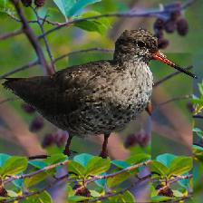
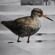
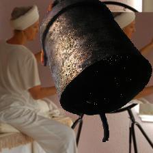
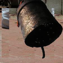
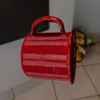
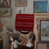
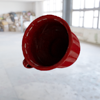
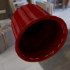
3DB lets us reproduce these findings effortlessly and without introducing such artifacts. To demonstrate this, we use 3DB to render our mug 3D model on hundreds of HDRI backgrounds, resulting in images such as:

We then analyze the performance of a pretrained ResNet-18Recall that this model obtains 42% accuracy on the corresponding "coffee mug" ImageNet class subset.on these images. We find that the performance of the classifier varies significantly across backgrounds, and that accuracy correlates with a crude measure of “background simplicity” (the JPEG compressed size of the image—with smaller size corresponding to being more simple).

A note on compositionality: An important part of 3DB that we don’t discuss here is compositionality, i.e., the ability to put together multiple controls and study their joint effect. For example, in our paper we studied how a model’s prediction vary with various zoom levels and backgrounds of an object. We found that the optimal zoom level varies a lot by background.

# $BLENDER_DATA/blender_environments` contains several backgrounds and
# $BLENDER_DATA/blender_models contains the 3D model of a mug.
export BLENDER_DATA=$(realpath blog_demo)/data/backgrounds
# if you want to use the pre-written material in blog_demo, uncomment:
# cd blog_demo

# (Optional) Download additional backgrounds you want---e.g., from
# https://hdrihaven.com/hdris/ (both `.hdr` and `.blend` files work) and put
# them in BLENDER_DATA/blender_environments. 
wget https://hdrihaven.com/hdris/PATH/TO/HDRI \
    -O $BLENDER_DATA/blender_environments

# Direct results
export RESULTS_FOLDER='results_backgrounds'

# Run 3DB (with the YAML file from the next pane saved as `backgrounds.yaml`):
threedb_workers 1 $BLENDER_DATA 5555 > client.log &
threedb_master $BLENDER_DATA backgrounds.yaml $RESULTS_FOLDER 5555

# Analyze results in the dashboard
python -m threedboard $RESULTS_FOLDER --port 3000
# Navigate to localhost:3000 to view the results!

# Finally, run analysis using pandas (third pane)
python analyze_bgs.py

base_config: "base.yaml"
policy:
  module: "threedb.policies.random_search"
  samples: 20
controls:
  - module: "threedb.controls.blender.orientation"
  - module: "threedb.controls.blender.camera"
    zoom_factor: [0.7, 1.3]
    aperture: 8.
    focal_length: 50.
  - module: "threedb.controls.blender.denoiser"

import pandas as pd
import numpy as np
import json

log_lines = open('results_backgrounds/details.log').readlines()
class_map = json.load(open('results_backgrounds/class_maps.json'))
df = pd.DataFrame.from_records(list(map(json.loads, log_lines)))
df['prediction'] = df['prediction'].apply(lambda x: class_map[x[0]])
df['is_correct'] = (df['is_correct'] == 'True')

res = df.groupby('environment').agg(accuracy=('is_correct', 'mean'),
        most_frequent_prediction=('prediction', lambda x: x.mode()))
print(res)

Texture Bias

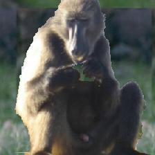
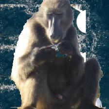
Another recent study of neural network biases showed that in contrast to humans, convolutional neural networks (CNNs) rely more on texture to recognize objects than on shape. The example below typifies this phenomenon—a cat with an elephant texture is recognized as a cat by humans, but as an elephant by CNNs:

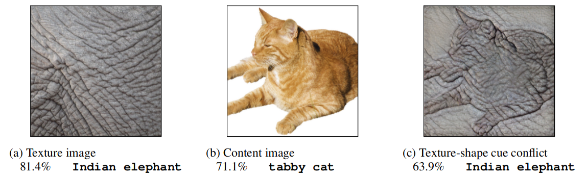
This example and others like it (dubbed ‘cue-conflict’ images) provide a striking illustration of the contrast between human and CNN-based classification mechanisms. Still, just as in the case of image backgrounds, creating such images typically necessitates time, technical skill, quality control, and/or introduction of unwanted artifacts (for example, in the above figure, ideally we would modify only the texture of the cat without altering the background).

However, using 3DB we can easily collect photorealistic empirical evidence of texture bias. Without modifying the internal 3DB codebase at all, one can write a custom control that modifies the texture of objects in the scene while keeping the rest intact. With this custom control in placeIn fact, the texture-swapping control for this experiment is now pre-packaged with 3DB, since we already wrote it ourselves!, one can simply randomize the texture of the mug across various backgrounds, poses and camera parameters before stratifying results:

Choose an Image

Average accuracy (compare to 42% on ImageNet val set)

The performance of the pretrained model on mugs (and other objects) deteriorates severely upon replacing the mug’s texture with a “wrong” one, providing clear corroborating evidence of the texture bias! We noticed in our experiments that for some textures (e.g., zebra), the coffee mug was consistently misclassified as the corresponding animal, whereas for others (e.g., crocodile), the mug is misclassified as either a related class (e.g., turtle or other reptile), or as an unrelated object (e.g., a trash can).

# ${BLENDER_DATA}/blender_environments contains several backgrounds,
# ${BLENDER_DATA}/blender_models contain the 3D model of a mug.
export BLENDER_DATA=$(realpath blog_demo)/data/texture_swaps

# List the materials that we will use for this post:
ls blog_demo/data/texture_swaps/blender_control_material
# You can also make or download blender materials corresponding 
# to other textures you want to test, and add them to that folder 

# if you want to use the pre-written material in blog_demo, uncomment:
# cd blog_demo

export RESULTS_FOLDER=results_texture

# Run 3DB (with the YAML file from the next pane saved as texture_swaps.yaml):
threedb_workers 1 $BLENDER_DATA 5555 > client.log &
threedb_master $BLENDER_DATA texture_swaps.yaml $RESULTS_FOLDER 5555

# Analyze results in the dashboard
python -m threedboard $RESULTS_FOLDER --port 3000
# Navigate to localhost:3000 to view the results!

# Finally, run analysis using pandas (copy from third pane)
python analyze_ts.py

base_config: "base.yaml"
controls:
  - module: "threedb.controls.blender.orientation"
    rotation_x: -1.57
    rotation_y: 0.
    rotation_z: [-3.14, 3.14]
  - module: "threedb.controls.blender.position"
    offset_x: 0.
    offset_y: 0.5
    offset_z: 0.
  - module: "threedb.controls.blender.pin_to_ground"
    z_ground: 0.25
  - module: "threedb.controls.blender.camera"
    zoom_factor: [0.7, 1.3]
    view_point_x: 1.
    view_point_y: 1.
    view_point_z: [0., 1.]
    aperture: 8.
    focal_length: 50.
  - module: "threedb.controls.blender.material"
    replacement_material: ["cow.blend", "elephant.blend", "zebra.blend", "crocodile.blend", "keep_original"]
  - module: "threedb.controls.blender.denoiser"

import pandas as pd
import numpy as np
import json

log_lines = open('results_texture/details.log').readlines()
class_map = json.load(open('results_texture/class_maps.json'))
df = pd.DataFrame.from_records(list(map(json.loads, log_lines)))
df = df.drop('render_args', axis=1).join(pd.DataFrame(df.render_args.values.tolist()))
df['prediction'] = df['prediction'].apply(lambda x: class_map[x[0]])
df['is_correct'] = (df['is_correct'] == 'True')

res = df.groupby('MaterialControl.replacement_material').agg(acc=('is_correct', 'mean'),
      most_frequent_prediction=('prediction', lambda x: x.mode()))
print(res)

Part-of-Object Attribution

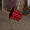
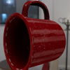
Beyond general hypotheses about model biases, 3DB allows us to test vision systems on a more fine-grained level. In the case of our running mug example, for instance, we can use the platform to understand which specific parts of its 3D mesh correlate with classifier accuracy. Specifically, below we generate (and classify) scenes with random mug positions, rotations, and backgrounds. Since 3DB stores texture-coordinate information for each rendering, we can reconstruct a three-dimensional heatmap that encodes, for each point on the surface of the mug, the classifier’s accuracy conditioned on that point being visible:

A number of phenomena stand out from this heatmap, including:

1. The classifier is worse when the side of the mug opposite the handle is seen.
2. The classifier is more accurate when the bottom rim is visible.
3. The classifier performs worst when the inside of the mug is visible.

# point BLENDER_DATA to the environments and models for this experiment
export BLENDER_DATA=$(realpath blog_demo)/data/part_of_object
# if you want to use the pre-written material in blog_demo, uncomment:
# cd blog_demo

# Optionally: download additional backgrounds (`.hdr` or `.blend`) e.g.,
wget URL -O $BLENDER_DATA/blender_environments/new_env.hdr

# Point results folder to where you want output written
export RESULTS_FOLDER='results_part_of_object'

# Run 3DB (with the YAML file from the next pane):
threedb_workers 1 $BLENDER_DATA 5555 > client.log &
threedb_master $BLENDER_DATA part_of_object.yaml $RESULTS_FOLDER 5555

# Analyze results in the dashboard
python -m threedboard $RESULTS_FOLDER --port 3000
# Navigate to localhost:3000 to view the results!

# Run `part_of_object.py` (third pane) to generate the heat map of the mug.
python po_analysis.py

base_config: "base.yaml"
policy:
  module: "threedb.policies.random_search"
  samples: 20
render_args:
  engine: 'threedb.rendering.render_blender'
  resolution: 256
  samples: 16
  with_uv: True
controls:
  - module: "threedb.controls.blender.orientation"
    rotation_x: -1.57
    rotation_y: 0.
    rotation_z: [-3.14, 3.14]
  - module: "threedb.controls.blender.camera"
    zoom_factor: [0.7, 1.3]
    view_point_x: 1.
    view_point_y: 1.
    view_point_z: 1.
    aperture: 8.
    focal_length: 50.
  - module: "threedb.controls.blender.denoiser"
  - module: "threedb.controls.blender.background"
    H: 1.
    S: 0.
    V: 1.

import pandas as pd
import numpy as np
import json
from PIL import Image

DIR = 'results_part_of_object'
log_lines = open(f'{DIR}/details.log').readlines()
df = pd.DataFrame.from_records(list(map(json.loads, log_lines)))

# From class index to class name (for readability)
class_map = json.load(open(f'{DIR}/class_maps.json'))
df['prediction'] = df['prediction'].apply(lambda x: class_map[x[0]])

# We'll be a little lenient here to get a more interesting heatmap
df['is_correct'] = df['prediction'].isin(['cup', 'coffee mug'])

uv_num_correct = np.zeros((256, 256))
uv_num_visible = np.zeros((256, 256))
for imid in df["id"].unique().tolist():
    is_correct = float(df.set_index('id').loc[imid]['is_correct'])
    vis_coords_im = Image.open(f'{DIR}/images/{imid}_uv.png')
    vis_coords = np.array(vis_coords_im).reshape(-1, 3)
    # R and G channels encode texture coordinates (x, y), 
    # B channel is 255 for object and 0 for background
    # So we will filter by B then only look at R and G.
    vis_coords = vis_coords[vis_coords[:,2] > 0][:,:2]

    uv_num_visible[vis_coords[:,0], vis_coords[:,1]] += 1.
    uv_num_correct[vis_coords[:,0], vis_coords[:,1]] += is_correct

# Accuracy = # correct / # visible
uv_accuracy = uv_num_correct / (uv_num_visible + 1e-4)

# Saves a black-and-white heatmap
Image.fromarray((255 * uv_accuracy).astype('uint8'))

Now that we have hypotheses regarding model performance, we can test them! Inspecting the ImageNet validation set, we found that our classifier indeed (a) struggles on coffee mugs when the handle is not showing (providing a feasible explanation for (1), since the side opposite the handle is only visible when the handle itself isn’t), and (b) performs worse at higher camera angles (providing a plausible explanation for (2)). We want to focus, however, on the third phenomenon, i.e., that the classifier performs quite poorly whenever the inside of the mug is visible. Why could this be the case? We can use 3DB to gain insight into the phenomenon. Specifically, we want to test the following hypothesis: when classifying mugs, does our ImageNet model rely on the exact liquid inside the cup?

We investigate this hypothesis by writing a custom control that fills our mug with various liquids (more precisely, a parameterized mixture of water, milk, and coffee):

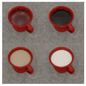
In contrast to the last experiment (where we varied the orientation of the mug), we render scenes containing the mug in a fixed set of poses that reveal the contents—just as in the last experiment, however, we still vary background and mug location. We visualize the results below—each cell in the heatmap corresponds to a fixed mixture of coffee, water, and milk (i.e., the labeled corners are 100% coffee, 100% milk, and 100% water, and the other cells are linear interpolations of these ratios) and the color of the cell encodes the relative accuracy of the classifier when the mug is filled with that liquid:

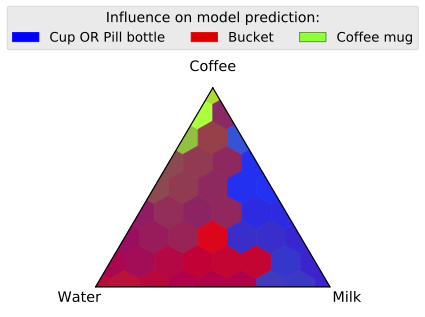
It turns out that mug content indeed highly impacts classification: our model is much less likely to correctly classify a mug that doesn’t contain coffee! This is just one example of how 3DB can help in proving or disproving hypotheses about model behavior.

From Simulation to Reality

So far, we’ve used 3DB to discover ML models’ various failure modes and biases via photorealistic rendering. To what extent though do the insights gleaned from simulated 3DB experiments actually “transfer” to the physical world?

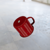
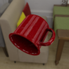
To test such transferability, we began by creating a 3D model of a physical room we had access to. We also collected eight different 3D models with closely matching physical world counterparts—including the mug analyzed above. Next, we used 3DB to find correctly and incorrectly classified configurations (pose, orientation, location) of these eight objects inside that room. Finally, we replicated these poses (to the best of our abilities) in the physical room, and took photos with a cellphone camera:

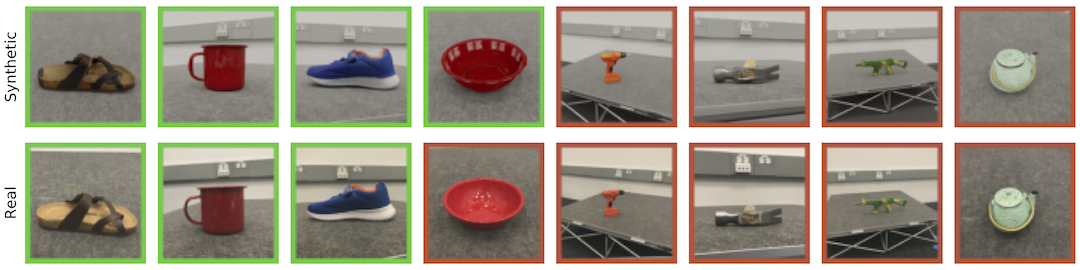
We classified these photos with the same vision model as before and measured how often the simulated classifier correctness matched correctness on the real photographs. We observed an ~85% match! So the failure modes identified by 3DB are not merely simulation artifacts, and can indeed arise in the real world.

Conclusion

3DB is a flexible, easy-to-use, and extensible framework for identifying model failure modes, uncovering biases, and testing fine-grained hypotheses about model behavior. We hope it will prove to be a useful tool for debugging vision models.

Bonus: Object Detection, Web Dashboard, and more!

We’ll wrap up by highlighting some additional capabilities of 3DB that we didn’t get to demonstrate in this blog post:

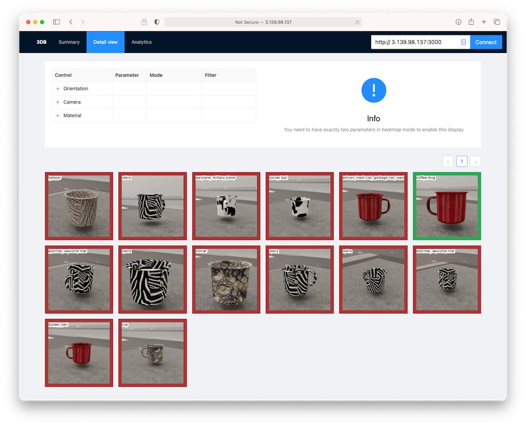
3DBoard: a web interface for exploring results

In all of the code examples above, we showed how to analyze the results of a 3DB experiment by loading the output into a pandas dataframe. For additional convenience, however, 3DB also comes with a web-based dashboard for exploring experimental results. The following command suffices to visualize the texture swaps experiment from earlier:

python -m threedboard results_texture/ --port 3000

Navigating to YOUR_IP:3000 should lead you to a page that looks like this:

Object detection and other tasks

In this blog post, we focused on using 3DB to analyze image classification models. However, the library also supports object detection out-of-the-box, and can easily be extended to support a variety of image-based tasks (e.g., segmentation or regression-based tasks). For example, below we provide a simple end-to-end object detection example:

# The object detection example is separate from the rest of the blog demo, so
# run the following in a separate repo:
git clone https://github.com/3db/object_detection_demo

# The repo has a data/ folder containing the Blender model (a banana) and some
# HDRI backgrounds, a classmap.json file mapping the UID of the model to a COCO
# class, and the detection.yaml file from the next pane.
cd object_detection_demo/

export BLENDER_DATA=data/
export RESULTS_FOLDER=results/

# Run 3DB
threedb_workers 1 $BLENDER_DATA 5555 > client.log & 
threedb_master $BLENDER_DATA detection.yaml $RESULTS_FOLDER 5555

# Analyze results in the dashboard
python -m threedboard $RESULTS_FOLDER --port 3000
# Navigate to localhost:3000 to view the results!

inference:
  module: 'torchvision.models.detection'
  class: 'retinanet_resnet50_fpn'
  label_map: './resources/coco_mapping.json'
  normalization:
    mean: [0., 0., 0.]
    std: [1., 1., 1.]
  resolution: [224, 224]
  args:
    pretrained: True
evaluation:
  module: 'threedb.evaluators.detection'
  args:
    iou_threshold: 0.5
    nms_threshold: 0.1
    max_num_boxes: 10
    classmap_path: 'classmap.json'
render_args:
  engine: 'threedb.rendering.render_blender'
  resolution: 256
  samples: 16
  with_segmentation: true
policy:
  module: "threedb.policies.random_search"
  samples: 2
logging:
  logger_modules:
    - "threedb.result_logging.image_logger"
    - "threedb.result_logging.json_logger"
controls:
  - module: "threedb.controls.blender.orientation"
  - module: "threedb.controls.blender.camera"
    zoom_factor: [0.7, 1.3]
    aperture: 8.
    focal_length: 50.
  - module: "threedb.controls.blender.denoiser"