Supervised deep learning is, by now, relatively stable from an engineering point of view. Training an image classifier on any dataset can be done with ease, and requires little of the architecture, hyperparameter, and infrastructure tinkering that was needed just a few years ago. Nevertheless, getting a precise understanding of how different elements of the framework play their part in making deep learning stable remains a challenge.
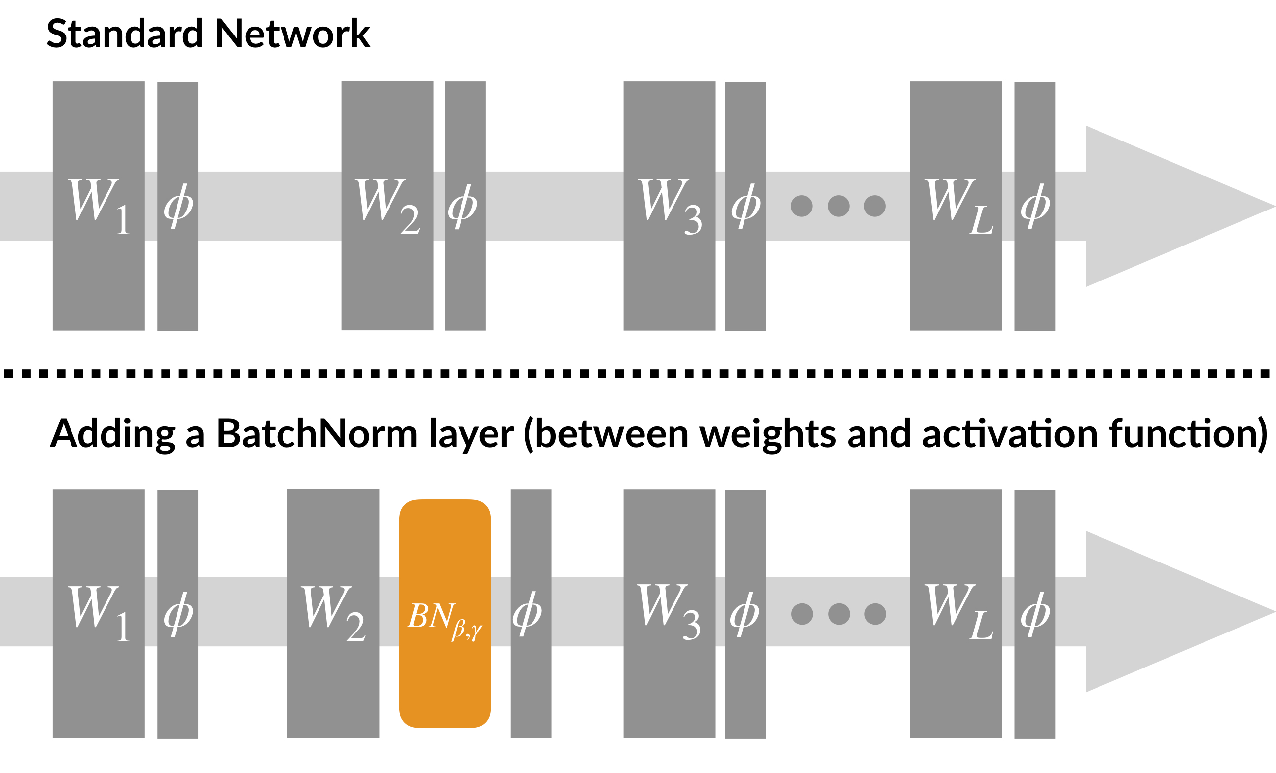
Today, we explore this challenge in the context of batch normalization (BatchNorm), one of the most widely used tools in modern deep learning. Broadly speaking, BatchNorm is a technique that aims to whiten activation distributions by controlling the mean and standard deviation of layer outputs (across a batch of examples). Specifically, for an activation \(y_j\) of layer \(y\), we have that:
\begin{equation} BN(y_j)^{(b)} = \gamma \cdot \left(\frac{y_j^{(b)} - \mu(y_j)}{\sigma(y_j)}\right) + \beta, \end{equation}
where \(y_j^{(b)}\) denotes the value of the output \(y_j\) on the \(b\)-th input of a batch, \(m\) is the batch size, and \(\beta\) and \(\gamma\) are learned parameters controlling the mean and variance of the output.
BatchNorm is also simple to implement, and can be used as a drop-in addition to a standard deep neural net architecture:
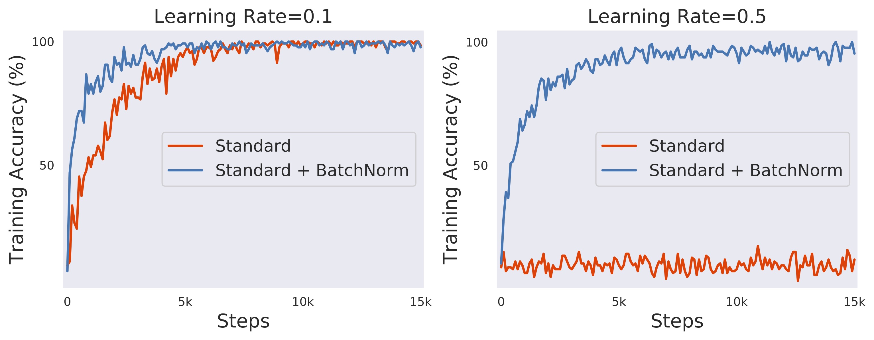
Now, it turns out that neural networks with BatchNorm tend to train faster, and are less sensitive to the choice of hyperparameters. Indeed, below we can see that, compared to its standard (i.e., unnormalized) variant, a VGG network with BatchNorm (on CIFAR10): (a) converges faster (even if we tune the learning rate in the unnormalized case), and (b) successfully trains even for learning rates for which the standard variant diverges.
In light of the above, it should not come as a surprise that BatchNorm has gained enormous popularity. The BatchNorm paper has over seven thousand citations (and counting), and is included by default in almost all “prepackaged” deep learning model libraries.
Despite this pervasiveness, however, we still lack a good grasp of why exactly BatchNorm works. Specifically, we don’t have a concrete understanding of the mechanism which drives its effectiveness in neural network training.
The story so far
The original BatchNorm paper motivates batch normalization by tying it to a phenomenon known as internal covariate shift. To understand this phenomenon, recall that training a deep network can be viewed as solving a collection of separate optimization problems - each one corresponding to training a different layer:
Now, during training, each step involves updating each of the layers simultaneously. As a result, updates to earlier layers cause changes in the input distributions of later layers. This implies that the optimization problems solved by subsequent layers change at each step.
These changes are what is referred to as internal covariate shift.
The hypothesis put forth in the BatchNorm paper is that such constant changes in layers’ input distribution force the corresponding optimization processes to continually adapt, thereby hampering convergence. And batch normalization was proposed exactly to alleviate this effect, i.e., to reduce internal covariate shift (by controlling the mean and variance of input distributions), thus allowing for faster convergence.
A closer look at internal covariate shift
At first glance, the above motivation seems intuitive and appealing—but is it actually the main factor behind BatchNorm’s effectiveness? In our recent paper, we investigate this question.
Our point of start is taking a closer look at training a deep neural network—how does training with and without BatchNorm differ? In particular, can we capture the resulting reduction in internal covariate shift?
To this end, let us examine both the standard and batch normalized variants of the VGG network, and plot a histogram of activations at various layers. (Note that each distribution constitutes the input of the optimization problem corresponding to the subsequent layer.)
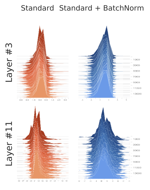
We can see that the activations of the batch normalized network seem controlled, and relatively stable between iterations. This is as expected. What is less expected, however, is that when we look at the network without BatchNorm, we don’t see too much instability either. Even without explicitly controlling the mean and variance, the activations seem fairly consistent.
So, is reduction of internal covariate shift really the key phenomenon at play here?
To tackle this question, let us first go back and take another look at our core premise: is the notion of internal covariate shift we discussed above actually detrimental to optimization?
Internal covariate shift & optimization: a simple experiment
Thus far, our focus was on reducing internal covariate shift (or removing it altogether): what if instead, we actually increased it? In particular, in a batch normalized network, what if we add non-stationary Gaussian noise (with a randomly sampled mean and variance at each iteration) to the outputs of the BatchNorm layer? (Note that by doing this, we explicitly remove the control that BatchNorm typically has over the mean and variance of layer inputs.) Below, we visualize the activations of such “noisy BatchNorm” (using the same methodology we used earlier):
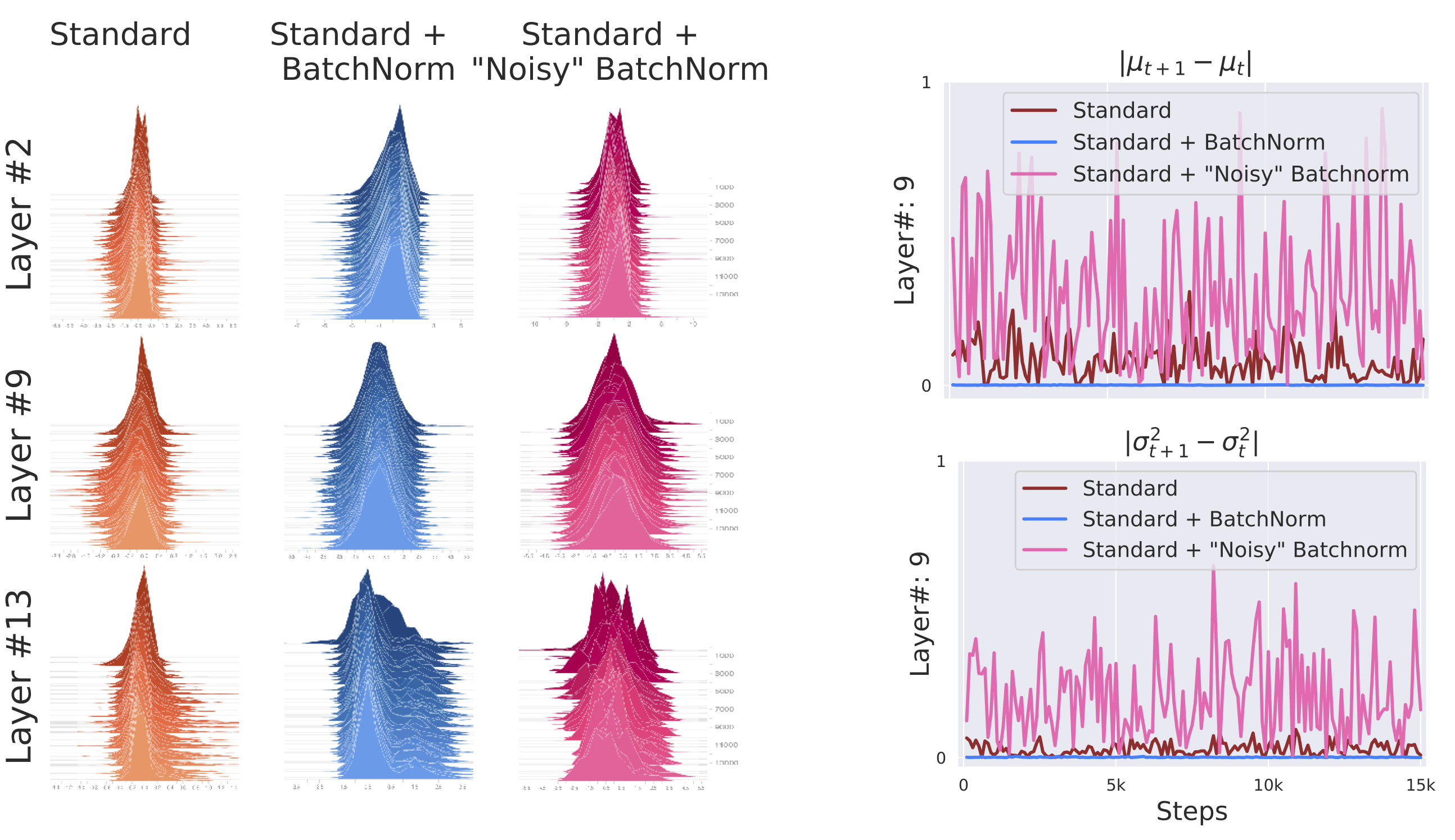
We can see that the activations of “noisy” BatchNorm are noticeably unstable, even more so than those of an unnormalized network. (Plotting the mean and variance of these distributions makes this even more apparent.)
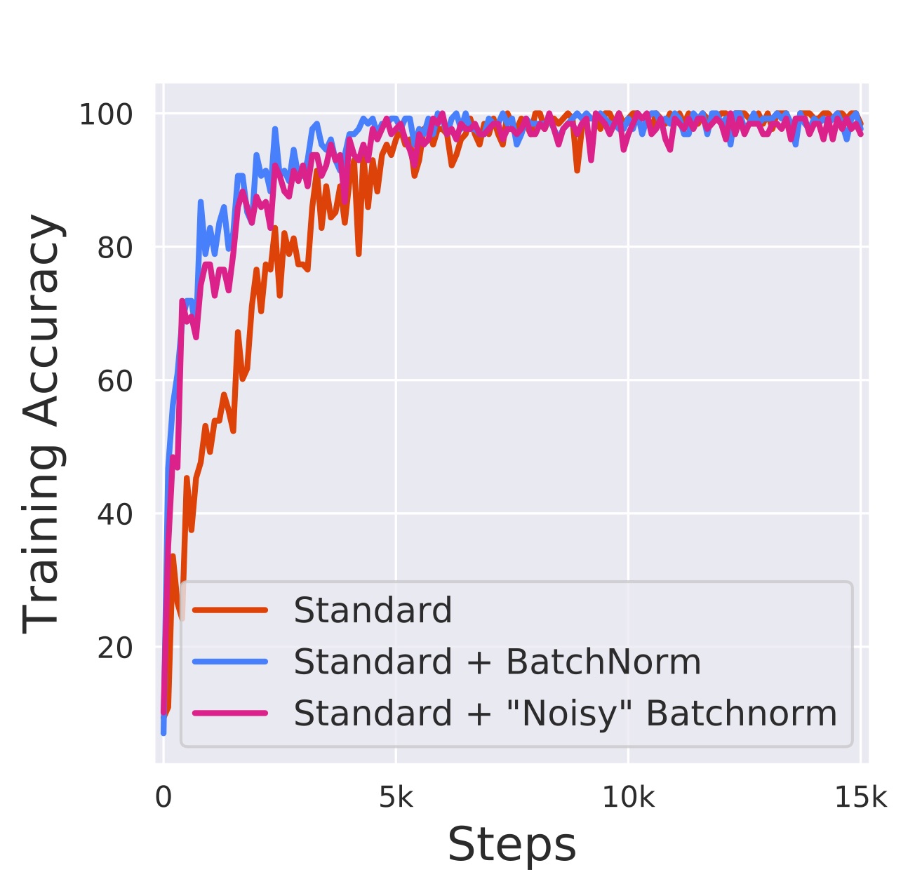
Remarkably, however, optimization performance seems to be unaffected. Indeed, in the graph below, we see that a network with noisy BatchNorm converges significantly faster compared to the standard network (and around the same speed as a network with the conventional batch normalization):
The above experiment may bring into question the connection between internal covariate shift and optimization performance. So, maybe there is a better way to cast this connection?
An optimization-based view on internal covariate shift
The original interpretation of internal covariate shift focuses on the distributional view of the stability the inputs. However, since our interest revolves around optimization, perhaps there is a different notion of stability—a one more closely connected to optimization—that BatchNorm enforces?
Recall that the intuition suggesting a connection between internal covariate shift and optimization was that constant changes to preceding layers interfere with the layer’s convergence. Thus, a natural way to quantify these changes would be via measuring the extent to which they affect the corresponding optimization problem. More specifically, given that our networks are optimized using (stochastic) first-order methods, the object of interest would be the gradient. This leads to an alternative, “optimization-oriented” notion of internal covariate shift. This notion defines internal covariate shift as the change in gradient direction of a layer caused by updates to preceding layers:
Definition. If \(w_{1:n}\) and \(w'_{1:n}\) are the parameters of an \(n\)-layer network before and after a single gradient update (respectively), then we measure the (optimization-based) internal covariate shift at layer \(k\) as \begin{equation} ||\nabla_{w_k}\mathcal{L}(w_{1:n}) - \nabla_{w_k} \mathcal{L}(w’_{1:k-1}, w_{k:n})||, \end{equation} where \(\mathcal{L}\) is the loss of the network.
Note that this definition quantifies exactly the discrepancy that was hypothesized to negatively impact optimization. Consequently, if BatchNorm is indeed reducing the impact of preceding layer updates on layer optimization, one would expect the above, optimization-based notion of internal covariate shift to be noticeably smaller in batch-normalized networks.
Surprisingly, when we measure the corresponding change in gradients (both in \(\ell_2\) norm and cosine distance), we find that this is not the case:
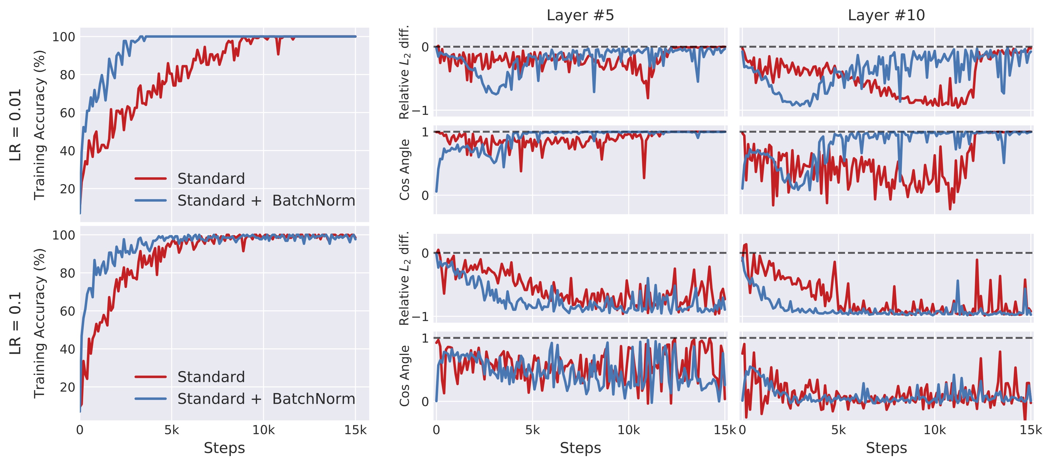
In fact, the change in gradients resulting from preceding layer updates appears to be virtually identical between standard and batch-normalized networks. (This persists, and is sometimes even more pronounced, for other learning rates and architectures.) Nevertheless, in all these experiments the batch-normalized network consistently achieves significantly faster convergence, as usual.
The impact of batch normalization
The above considerations might have undermined our confidence in batch normalization as a reliable technique. But BatchNorm is (reliably) effective. So, can we uncover the roots of this effectiveness?
Since we were unable to substantiate the connection between reduction of internal covariate shift and the effectiveness of BatchNorm, let us take a step back and approach the question from first principles.
After all, our overarching goal is to understand how batch normalization affects the training performance. It would be thus natural to directly examine the effect that BatchNorm has on the corresponding optimization landscape. To this end, recall that our training is performed using gradient descent method and this method draws on the first-order optimization paradigm. In this paradigm, we use the local linear approximation of the loss around the current solution to identify the best update step to take. Consequently, the performance of these algorithms is largely determined by how predictive of the nearby loss landscape this local approximation is.
Let us thus take a closer look at this question and, in particular, analyze the effect of batch normalization on that predictiveness. More precisely, for a given point (solution) on the training trajectory, we explore the landscape along the direction of the current gradient (which is exactly the direction followed by the optimization process). Concretely, we want to measure:
- Variation of the value of the loss: \begin{equation} \mathcal{L}(x + \eta\nabla \mathcal{L}(x)), \qquad \eta \in [0.05, 0.4]. \end{equation}
- Gradient predictiveness, i.e., the change of the loss gradient: \begin{equation} ||\nabla \mathcal{L}(x) - \nabla \mathcal{L}(x+\eta\nabla \mathcal{L}(x))||, \qquad \eta \in [0.05, 0.4]. \end{equation}
(Note that the typical learning rate used to train the network is \(0.1\).)
Below we plot the range of these quantities over the corresponding intervals at different points of the training trajectory:
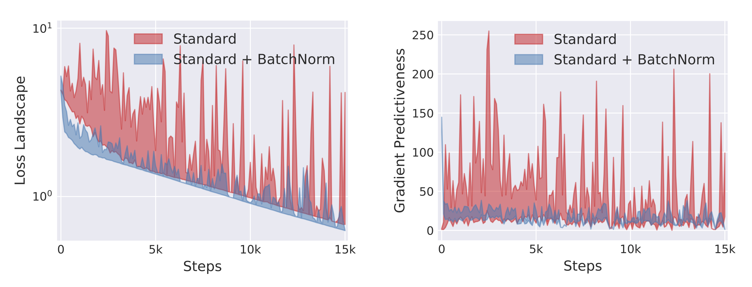
As we can see, adding a BatchNorm layer has a profound impact across both our metrics.
This impact might finally hint at the possible roots of BatchNorm’s effectiveness. After all, a small variability of the loss indicates that the steps taken during training are unlikely to drive the loss uncontrollably high. (This variability also reflects, in a way, the Lipschitzness of the loss.) Similarly, good gradient predictiveness implies that the gradient evaluated at a given point stays relevant over longer distances, hence allowing for larger step sizes. (This predictiveness can be seen as related to the \(\beta\)-smoothness of the loss.)
So, the “smoothing” effect of BatchNorm makes the optimization landscape much easier to navigate, which could explain the faster convergence and robustness to hyperparameters observed in practice.
BatchNorm reparametrization
The above smoothing effect of BatchNorm was evident in all experiments we performed. Can we understand though what is the fundamental phenomenon underlying it?
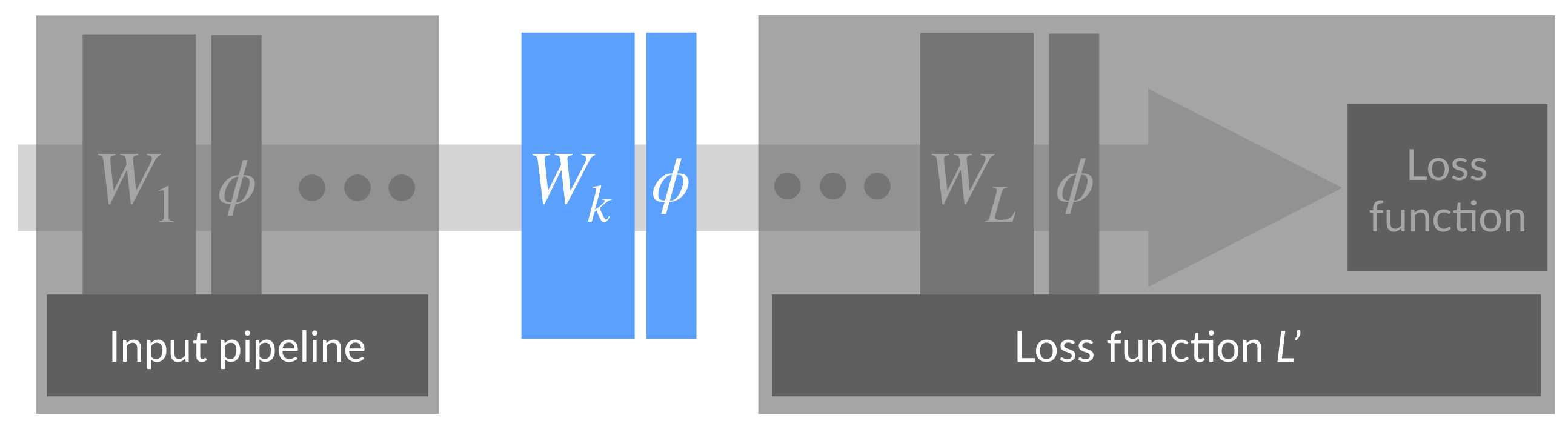
To this end, we formally analyzed a scenario where we add a single BatchNorm layer after a single layer of a deep network, and compared it to a case without BatchNorm:
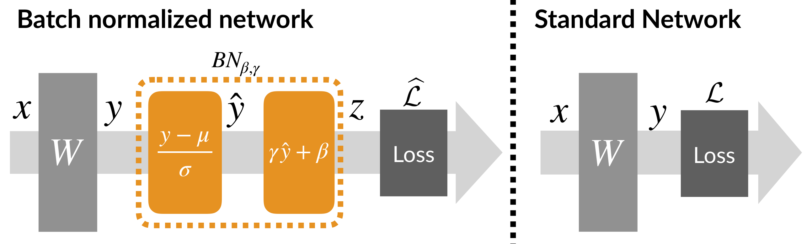
Note that this setup is quite general, since the input \(x\) could be the output of (an arbitrary number of) previous layers and the loss \(\mathcal{L}\) might incorporate an arbitrary number of subsequent layers.
We prove that BatchNorm effectively reparametrizes the training problem, making it more amenable to first-order methods. Specifically, batch normalization makes the optimization wrt the activations \(y\) easier. This, in turn, translates into improved (worst-case) bounds for the actual optimization problem (which is wrt the weights \(W\) and not the activations \(y\)).
More precisely, by unraveling the exact backwards pass induced by BatchNorm layer, we show that
Theorem 1. Let \(g = \nabla_y \mathcal{L}\) be the gradient of the loss \(\mathcal{L}\) wrt a batch of activations \(y\), and let \(\widehat{g} = \nabla_y \widehat{\mathcal{L}}\) be analogously defined for the network with (a single) BatchNorm layer.
We have that
\begin{equation}
||\widehat{g}||^2 \leq \frac{\gamma^2}{\sigma_j^2}\left(||g||^2 - \mu(g)^2 - \frac{1}{\sqrt{m}}\langle g, \widehat{y}\rangle^2\right).
\end{equation}
So, indeed, inserting the BatchNorm layer reduces the Lipschitz constant of the loss wrt \(y\). The above bound can be also translated into a bound wrt the weights \(W\) (which is what the optimization process actually corresponds to) in the setting where the inputs are set in a worst-case manner, i.e., so as to maximize the resulting Lipschitz constant. (We consider this setting to rule out certain pathological cases, which can, in principle, arise as we are making no assumptions about the input distribution. Alternatively, we could just assume the inputs are Gaussian.)
We can also corroborate our observation that batch normalization makes gradients more predictive. To this end, recall the Taylor series expansion of a function around a value \(x\): \begin{equation} \mathcal{L}(y+\Delta y) = \mathcal{L}(y) + \nabla \mathcal{L}(y)^\top \Delta y + \frac{1}{2}(\Delta y)^\top H (\Delta y) + o(||\Delta y||^2), \end{equation} where \(H\) is the Hessian matrix of the loss, and in our case \(\Delta y\) is a step in the gradient direction. We can prove that, under some mild assumptions, adding a BatchNorm layer makes the second-order term in that expansion smaller, thus increasing the radius in which the first-order term (the gradient) is predictive:
Theorem 2. Let \(H\) be the Hessian matrix of the loss wrt the a batch of activations \(y\) in the standard network and, again, let \(\widehat{H}\) be defined analogously for the network with (a single) BatchNorm layer inserted.
We have that
\begin{equation}
\widehat{g}^\top \widehat{H} \widehat{g}
\leq
\frac{\gamma^2}{\sigma^2}\left(
g^\top H g -
\frac{1}{m\gamma}\langle g, \widehat{y} \rangle ||\widehat{g}||^2
\right)
\end{equation}
Again, this result can be translates into an analogous bound wrt \(W\) in the setting where the inputs are chosen in a worst-case manner.
Looking forward
Our investigation so far has shed some light on the possible roots of BatchNorm’s effectiveness, but there is still much to be understood. In particular, while we identified the increased smoothness of the optimization landscape as a direct result of employing BatchNorm layers, we still lack a full grasp of how this impacts the actual training process.
Moreover, in our considerations we completely ignored the positive impact that batch normalization has on generalization. Empirically, BatchNorm often improves test accuracy by a few percentage points. Can we uncover the precise mechanism behind this phenomenon?
More broadly, we hope that our work motivates us all to take a closer look at other elements of our deep learning toolkit. After all, only once we attain a meaningful and more fine-grained understanding of that toolkit we will know the ultimate power and fundamental limitations of the techniques we use.
P.S. We will be at NeurIPS’18! Check out our 3-minute video and our talk on Tuesday.