This is the second part of the overview of our recent work on training more debuggable deep networks. In our previous post, we outlined our toolkit for constructing such networks, which involved training (very) sparse linear classifiers on (pre-trained) deep feature embeddings and viewing the network’s decision process as a linear combination of these features. In this post, we will delve deeper into evaluating to what extent these networks are amenable to debugging. Specifically, we want to get a sense of whether humans are able to intuit their behavior and pinpoint their failure modes.
Do our sparse decision layers truly aid human understanding?
Although our toolkit enables us to greatly simplify the network’s decision layer (by reducing the number of its weights and thus the features it relies on), it is not immediately obvious whether this will make debugging such models significantly easier. To properly examine this, we need to factor humans into the equation. One way to do that is to leverage the notion of simulatibility used in the context of ML interpretability. According to this notion, an interpretability method is “good” if it can enable a human to reproduce the model’s decision. In our setup, this translates into evaluating how sparsity of the final decision layer influences humans’ ability to predict the model’s classification decision (irrespective of whether this decision is “correct” or not).
The “simulatibility” study
One approach to assess simulatibility would be to ask annotators to guess what the model will label an input (e.g., an image) as, given an interpretation corresponding to that input. However, for non-expert annotators, this might be challenging due to the large number of (often fine-grained) classes that a typical dataset contains. Additionally, human cognitive biases may also muddle the evaluation—e.g., it may be hard for annotators to decouple “what they think the model should label the input as” from “what the interpretation suggests the model actually does” (and we are interested in the latter).
To alleviate these difficulties, we resort instead to the following task setup (conducted using an ImageNet-trained ResNet):
- We pick a target class at random, and show annotators visualizations of five randomly-selected features used by the sparse decision layer to detect objects of this class, along with their relative weights.
- We present the annotators with three images from the validation set with varying (but still non-trivial) probabilities of being classified by the model as the target class. (Note that each of these images can potentially belong to different, non-target classes.)
- Finally, we ask annotators to pick which one among these three images they believe to best match the target class.
Here is a sample task (click to enlarge):
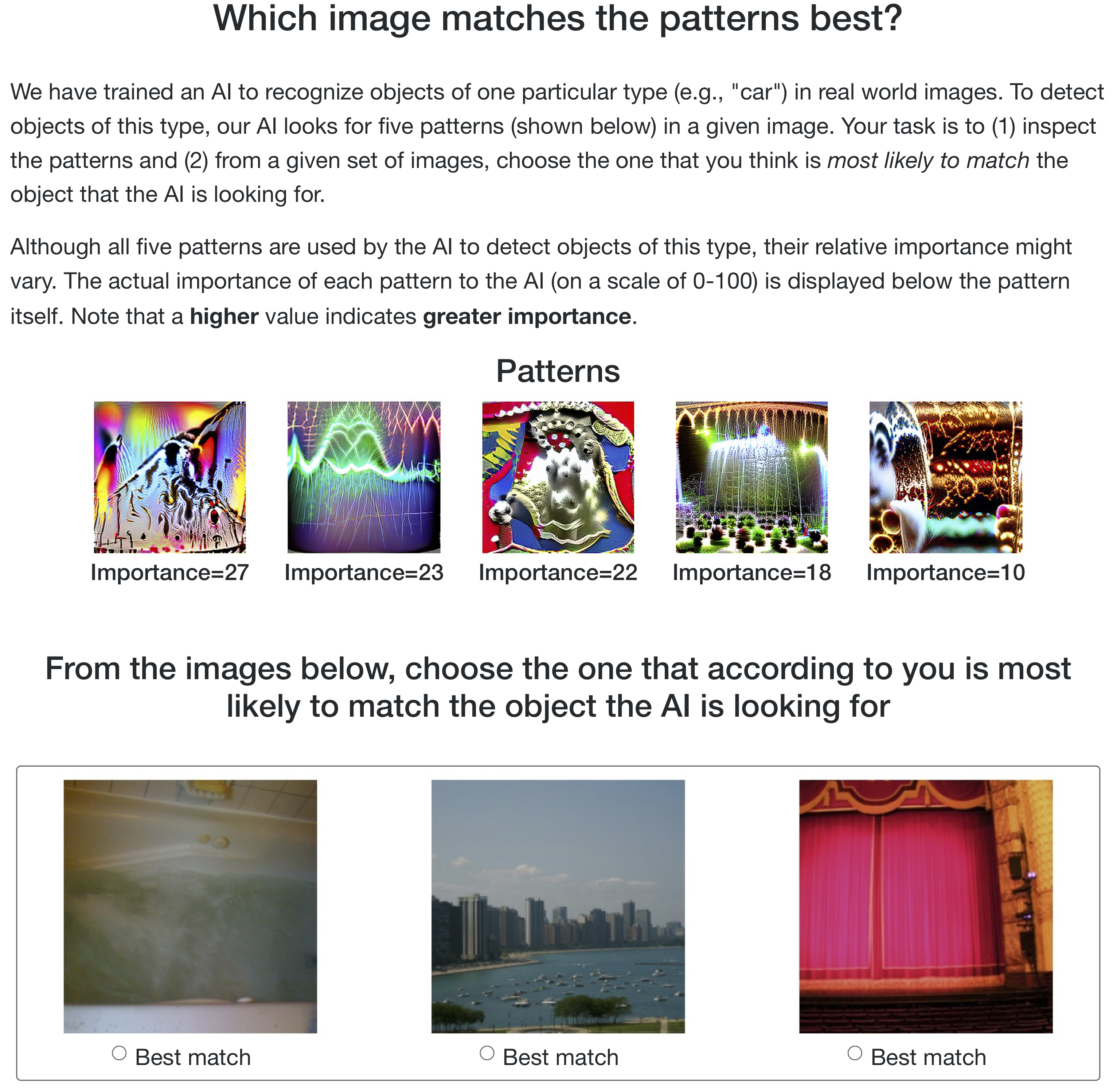
Overall, our intention is to gauge whether humans can intuit which image (out of three) is most prototypical for the target class according to the model. Note that we do not show annotators any information about the target class—such as its name or description—other than illustrations of some of the features that the model uses to identify it. As discussed previously, this is intentional: we want annotators to select the image that visually matches the features used by the model, instead of using their prior knowledge to associate images with the target label itself. For instance, if the annotators know that the target label was “car”, they might end up choosing the image that most closely resembles their idea of a car—independent of (or even in contradiction to) how the model actually detects cars. In fact, the “most activating image” in our setup may not even belong to the target class.
Now, how well do humans do on this task?
We find that (MTurk) annotators are pretty good at simulating the behavior of our modified networks—they correctly guess the top activating image (out of three) 63% of the time! In contrast, they essentially fail, with only a 35% success rate (i.e., near chance), when this task is performed using models with standard, i.e., dense, decision layers. This suggests that even with a very simple setup—showing non-experts some of the features the sparse decision layer uses to recognize a target class—humans are actually able to emulate the behavior of our modified networks.
Debuggability via Sparsity
So far, we identified a number of advantages of employing sparse decision layers, such as having fewer components to analyze, selected features being more influential, and better human simulatibility. But what unintended model behaviors can we (semi-automatically) identify by just probing such decision layers?
Uncovering (spurious) correlations and biases
Let’s start with trying to uncover model biases. After all, it is by now evident that deep networks rely on undesired correlations extracted from the training data (e.g. backgrounds, identity-related keywords). But can we pinpoint this behavior without resorting to a targeted examination?
Bias in toxic comment classification
In 2019, Jigsaw hosted a competition on Kaggle around creating toxic comment detection systems. This effort was prompted by that fact that the systems available at the time were found to have incorrectly learned to associate the names of frequently attacked identities (e.g., nationality, religion or sexual identity) with toxicity, and so the goal of the competition was to construct a “debiased” system. Can we understand to what extent this effort succeeded?
To answer this question we leverage our methodology and fit a sparse decision layer to the debiased model released by the contest organizers, and then inspect the utilized deep features. An example result is shown below:
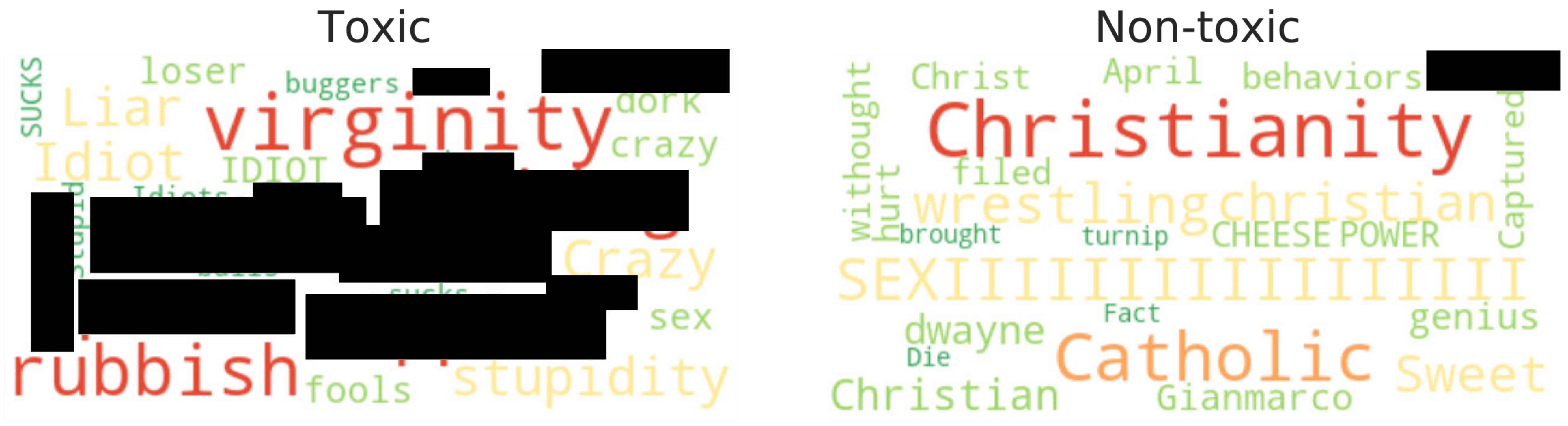
Looking at this visualization, we can observe that the debiased model no longer positively associates identity terms with toxicity (refer our paper for a similar visualization corresponding to the original biased model). This seems to be a success—after all, the goal of the competition was to correct the over-sensitivity of prior models to identity-group keywords. However, upon closer inspection, one will note that the model has actually learned a strong, negative association between these keywords and comment toxicity. For example, one can take a word such as “christianity” and append it to toxic sentences to trick the model into thinking that these are non-toxic 74% of the time. One can try it by selecting words to add to the sentence below:
So, what we see is that rather than being debiased, newer toxic comment detection systems remain disproportionately sensitive to identity terms—it is just the nature of the sensitivity that changed.
Spurious correlations in ImageNet
In the NLP setting, we can directly measure correlations between the model’s predictions and input data patterns by toggling specific words or phrases in the input corpus. However, it is not obvious how to replicate such analysis in the vision setting. After all, we don’t have automated tools to decompose images into a set of human understandable patterns akin to words or phrases (e.g., “dog ears” or “wheels”).
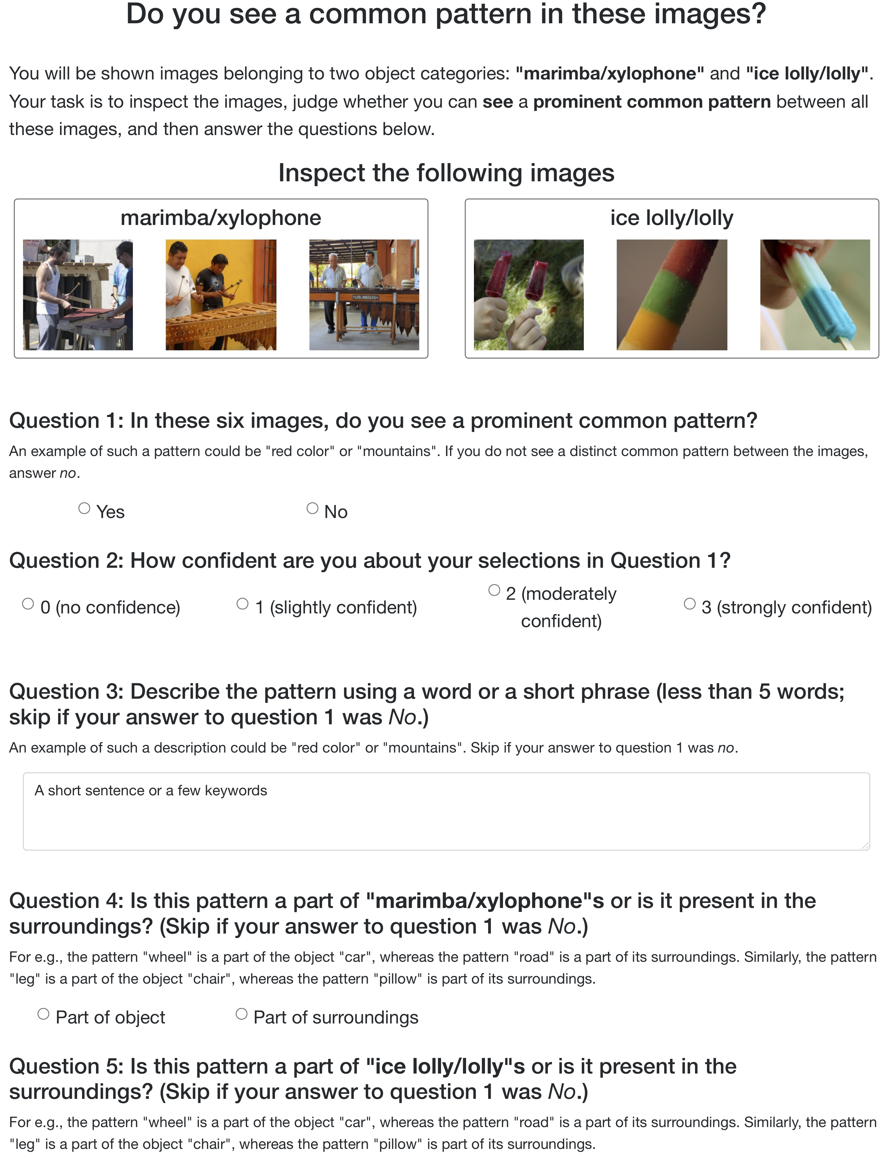
We thus leverage instead a human-in-the-loop approach that uses (sparse) decision layer inspection as a primitive. Specifically, we enlist annotators on MTurk to identify and describe data patterns that activate individual features that the sparse decision layer uses (for a given class). This in turn allows us to pinpoint the correlations the model has learned between the input data and that class.
Concretely, to identify the data patterns that are positively correlated with a particular (deep) feature, we present to MTurk annotators a set of images that strongly activate it. The expectation here is that if a set of images activate a given feature, these images should share a common input pattern and the annotators will be able to identify it.
We then ask annotators: (a) whether they see a common pattern in the images, and, if so, (b) to provide a free text description of that pattern. If the annotators identify a common input pattern, we also ask them if the identified pattern belongs to the class object (“spurious”) or its surroundings (“non-spurious”) for each of the two classes.
Here is an example of the annotation task (click to expand):
Here are a few examples of (spurious) correlations identified by annotators:
Note that, one can, in principle, use the same human-in-the-loop methodology to identify input correlations extracted by standard deep networks (with dense decision layers). However, since these models rely on a large number of (deep) features to detect objects of every class, this process can quickly become intractable (see our paper for details).
The above studies demonstrate that for typical vision and NLP tasks, sparsity in the decision layer makes it easier to look deeper into the model and understand what patterns it has extracted from its training corpus.
Creating effective counterfactuals
Our second approach for characterizing model failure modes uses the lens of counterfactuals. We specifically focus on counterfactuals that are (minor) variations of given inputs that prompt the model to make a different prediction. Counterfactuals can be very helpful from a debugging standpoint—they can confirm that specific input patterns are not just correlated with the model prediction but actually causally influence them. Additionally, such counterfactuals can be used to provide recourse to users—e.g., to let them realize what attributes (e.g., credit rating) they should change to get the desired outcome (e.g., granting a loan). We will now discuss how to leverage the correlations identified in the previous section to construct counterfactuals for models with sparse decision layers.
Language counterfactuals in sentiment classification
In sentiment classification, the task is to label a given sentence as having either positive or negative sentiment. Here, we consider counterfactuals via word substitution, effectively asking “what word could I have used instead to change the sentiment predicted by the model for a given sentence?”
To this end, we consider the words that are positively and negatively correlated with features used by the sparse decision layer as candidates for word substitution. For example, the word “astounding” activates a feature that a BERT model uses to detect positive sentiment, whereas the word “condescending” is negatively correlated with the activation of this feature. By substituting such a positively-correlated word with its negatively-correlated counterpart, we can effectively “flip” the corresponding feature. A demonstration of this process is shown below:
| Positive activation | ||
|---|---|---|
| impressed | brings | marvel |
| exhilirated | astounding | completes |
| hilariously | successfully | yes |
| Negative activation | ||
|---|---|---|
| idiots | inconsistent | maddening |
| cheat | condescending | failure |
| dahmer | pointless | unseemly |
It turns out that these one-word modifications are indeed already quite successful (i.e., they cause a change in the model’s prediction 73% of the time). The obtained sentence pairs—which can be viewed as counterfactuals for one another—allow us to gain insight into data patterns that cause the model to predict a certain outcome. Finally, we find that for standard models finding effective counterfactuals that flip the model’s prediction is harder—the one-word modifications described above can only change the model’s decision in 52% of cases.
ImageNet counterfactuals
For ImageNet-trained models, we can directly use the patterns previously identified by the annotators to generate counterfactual images that change its prediction. To this end, we manually modify images to add or subtract these patterns and observe the effect of this operation on the model’s decision.
For example, annotators identify a background feature “chainlink fence” to be spuriously correlated with “ballplayers”. Using this information, we can then take images of people playing basketball or tennis (correctly labeled as “basketball” or “racket” by the model) and manually insert a “chainlink fence” into the background, which successfully changes the model’s prediction to “ballplayer”.
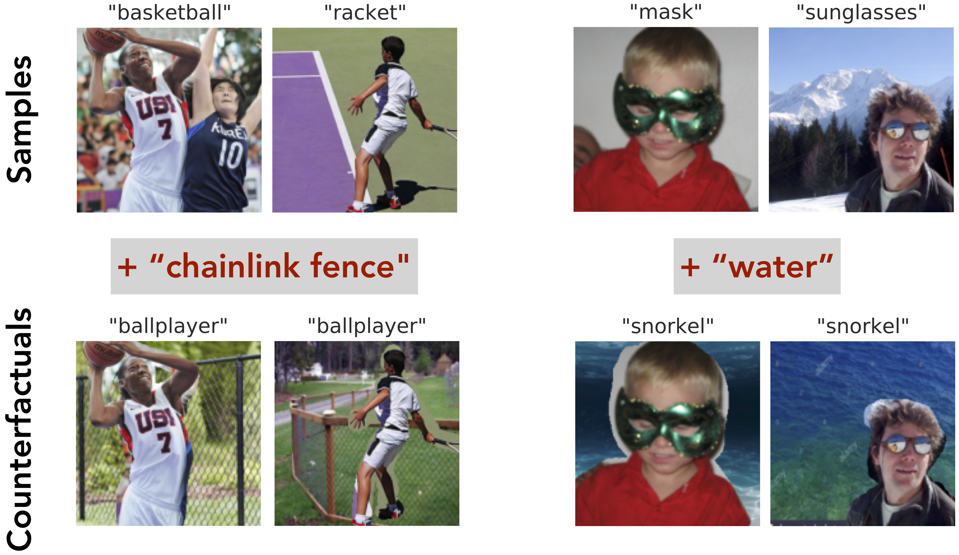
Thus, the counterfactuals that our methodology produced indeed allow us to identify data patterns that are causally linked to the model’s decision making process.
Identifying reasons for misclassification
Finally, we turn our attention to debugging model errors. After all, when our models are wrong, it would be helpful to know why this was the case.
In the ImageNet setting, we find that many (over 30%) of the misclassifications of the sparse-decision-layer models can be attributed to a single “problematic” feature. That is, manually removing this feature results in a correct prediction. One can thus view the feature interpretation for this problematic feature as a justification for the model’s error.
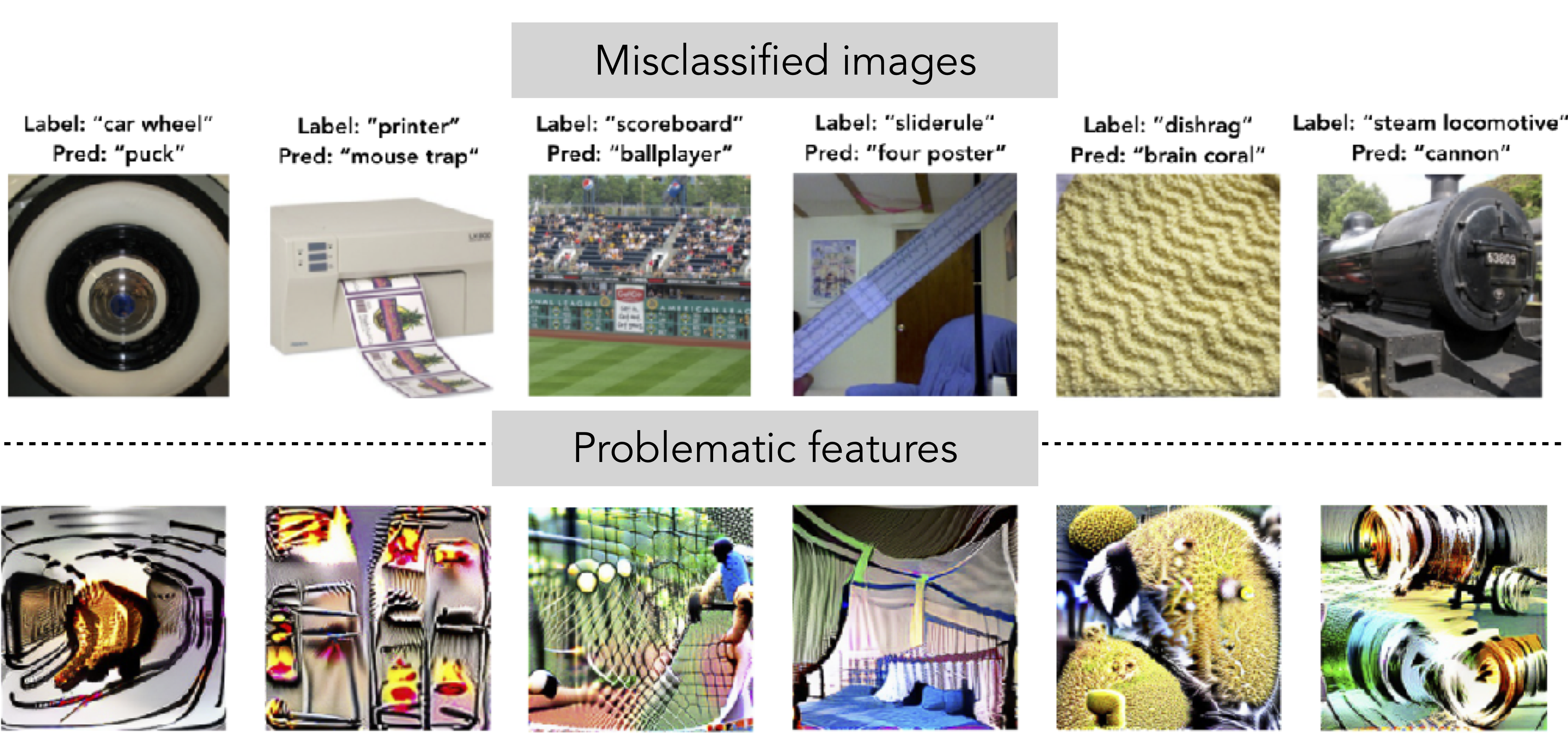
Ideally, given such a justification, we would like humans to be able to identify the part of the image corresponding to the problematic feature that caused the model to make a mistake. How can we evaluate whether this is the case? Namely, can we obtain an unbiased assessment of whether the data patterns that activate the problematic feature are noticeably present in the misclassified image?
To answer this question, we conduct a study on MTurk wherein we present annotators with an image, along with feature visualizations for: (i) the most activated feature from the true class and (ii) the problematic feature that is activated for the erroneous class. We do not explicitly tell the annotators what classes these features correspond to. We then ask annotators to select the patterns (feature visualizations) that match the image, and to determine which pattern is a better match if they select both.
Here is an example of a task we present to the annotators (click to expand):
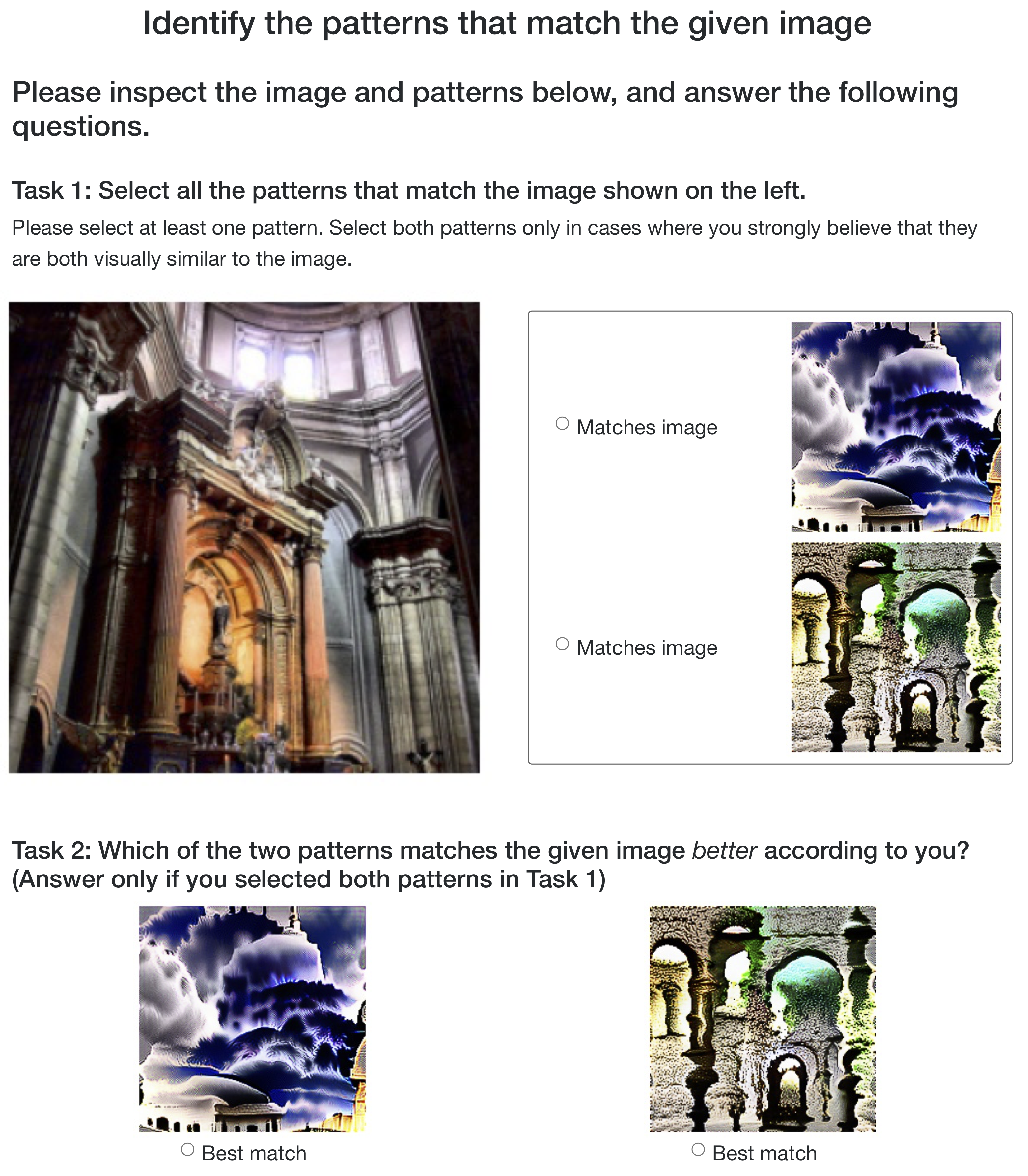
It turns out that not only do annotators frequently (70% of the time) identify the top feature from the wrongly-predicted class as present in the image, but also that this feature is actually a better match than the top feature for the ground truth class (60% of the time). In contrast, annotators select the control (randomly-chosen) deep feature to be a match for the image only 16% of the time. One can explore some examples here:
This experiment validates (devoid of confirmation biases from the class label) that humans can identify the data patterns that trigger the error-inducing problematic deep features. Note that once these patterns have been identified, one can examine them to better understand the root cause (e.g., issues with the training data) for model errors.
Conclusions
Over the course of this two-part series, we have shown that a natural approach of fitting sparse linear models over deep feature representations can already be surprisingly effective in creating more debuggable deep networks. In particular, we saw that models constructed using this methodology are more concise and amenable to human understanding—making it easier to detect and analyze unintended behaviors such as biases and misclassification. Going forward, this methodology of modifying the network architecture to make it inherently easier to probe can offer an attractive alternative to the existing paradigm of purely post-hoc debugging. Additionally, our analysis introduces a suite of human-in-the-loop techniques for model debugging at scale and thus can help guide further work in this field.