Deep reinforcement learning is behind some of the most publicized advances in machine learning, powering algorithms that can dominate human Go players and beat expert DOTA 2 teams. However, despite these successes, recent work has uncovered that deep reinforcement learning methods are plagued by training inconsistency, poor reproducibility, and overall brittleness.
These issues are troubling, especially in a field that has such an undeniable potential. What’s more troubling though is that with our current methods of evaluating RL algorithms, it might be hard to even detect these problems. Further, when we do detect them, we tend to get very little insight into what is happening under the hood.
Our recent work aims to take a step towards understanding this brittleness. Specifically, we take a re-look at current deep RL algorithms and ask: to what extent does the behavior of these methods line up with the conceptual framework we use to develop them?
In this three-part series (this is part 1, part 2 is here, and part 3 is here), we’ll walk through our investigation of deep policy gradient methods, a particularly popular family of model-free algorithms in RL. This part is meant to be an overview of the RL setup, and how we can use policy gradients to solve reinforcement learning problems. We’ll then discuss actual implementation of one of the most popular variants of these algorithms: proximal policy optimization (PPO).
Throughout the series, we’ll be introducing concepts and notation as we need them, keeping required background knowledge to a minimum.
The RL Setup
In the reinforcement learning setting we want to train an agent that interacts via actions with a stateful environment and its goal is to maximize total reward. In robotics, for example, we might have a humanoid robot (the agent) that actuates motors in its legs and arms (the actions), and attains a constant reward for staying upright (the reward). (In this example, the environment is really just the laws of physics.)
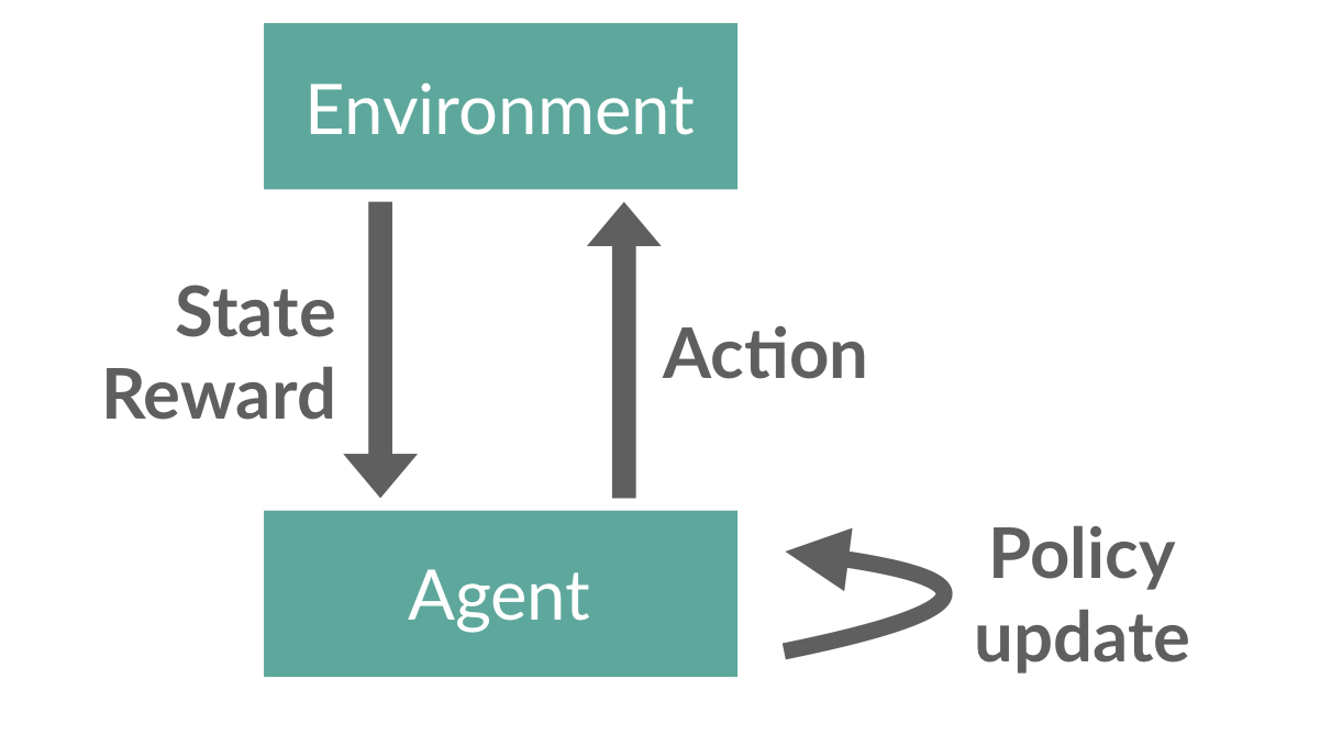
Concretely, introducing the notation with policy gradients (the algorithms we’re focusing on) in mind, we define the RL setting as follows. Agent behavior is specified by a policy function \(\pi\) that maps states (like the current position, in the robot example) to a probability distribution over possible actions to take. The agent interacts with the environment by repeatedly observing the current state \(s_t\); passing it to \(\pi\); sampling an action from \(\pi(\cdot\vert s_t)\); and, finally, receiving a reward \(r_t = r(s, a)\) and a next state \(s_{t+1}\). This repeated game stops when some pre-defined failure condition is met (e.g. the robot falls over) or after a certain predefined number of steps.
The entire interaction of the agent with the environment can be represented as a sequence of states, actions and rewards. This sequence is called a rollout, episode, or trajectory, and is typically denoted by \(\tau\). Then, \(r(\tau)\) is the total reward accumulated over that trajectory \(\tau\). Hence, more formally, the goal of a reinforcement learning is to find a policy which maximizes this total reward:
\begin{equation} \max_\pi \mathbb{E}_{\tau \sim \pi} \left[\sum_{(s,a) \in \tau} r(s, a) \right]. \end{equation}
So, how should we go about finding a policy that achieves this goal? One standard approach is to parameterize the policy by some vector \(\theta\), where \(\theta\) can be anything from entries in a table to weights in a neural network. (In the deep RL setting, we focus on the latter.) The policy induced by the parameter \(\theta\) is then usually denoted by \(\pi_\theta\).
The above parameterization allows us to rewrite the reinforcement learning objective in a clean new way. Specifically, our goal becomes to find \(\theta^*\) such that:
\begin{equation} \theta^* = \arg\max_\theta \mathbb{E}_{\tau \sim \pi_\theta} \left[\sum_{(s,a) \in \tau} r(s, a) \right]. \end{equation}
RL with Policy Gradients
Expressing our objective in the way above allows us to essentially view reinforcement learning purely as an optimization problem. This immediately suggests a natural way to maximize this objective: gradient descent (or really, gradient ascent).
However, it is unfortunately not that easy, as it’s unclear how to access the gradient of the objective above. In fact, this issue is precisely one of the key challenges in RL.
Is there a way to circumvent this difficulty? It turns out that we indeed can. To this end, we recall that first-order methods fare well even with estimates of the gradient. As a result, obtaining such an estimate is exactly what policy gradient methods do. To do so, it takes advantage of the following identity:
\begin{align} \tag{1} \label{eq:hello} g_\theta := \nabla_\theta \mathbb{E}_{\tau \sim \pi_\theta}[r(\tau)] = \mathbb{E}_{\tau \sim \pi_\theta} \left[ \nabla_\theta \log(\pi_\theta(\tau)) r(\tau)\right], \end{align} where \(g_\theta\) denotes the policy gradient we are interested in.
With some work (see the derivation below), we can simplify and manipulate this identity into a sort of “standard form” (which one might typically encounter, for example, in a presentation or textbook):
\begin{equation} \tag{2} \label{eq:pg} g_\theta = \mathbb{E}_{\tau \sim \pi_\theta} \left[ \sum_{t=1}^{|\tau|} \nabla_\theta \log(\pi_\theta(a_t|s_t)) Q^\pi(s_t, a_t)\right], \end{equation}
where \(Q^\pi(s_t, a_t) = \mathbb{E}[R_t\vert a_t, s_t, \pi]\) denotes the expected return from a policy that started in the state \(s_t\) and took first the action \(a_t\).
Now, we typically estimate the expectation above using a simple finite-sample mean. (Note that a rather nice way to think about this construction is that we sample some trajectories, and then try to increase the log-probability of the most successful ones.)
Implementing PPO
The policy gradient framework allows us to apply first-order techniques like gradient descent without having to differentiate through the environment. (This might remind us of zeroth-order optimization, and indeed there are interesting connections between the policy gradient and finite-difference techniques.)
Despite its elegance, however, in practice we rarely use the above form \eqref{eq:pg}. State-of-the-art algorithms employ instead several algorithmic refinements on top of the standard policy gradient. (We’ll go over these as we encounter them in the next few posts.)
So, let us consider one of the algorithms at the forefront of deep reinforcement learning: proximal policy optimization (PPO). Specifically, let us just start by taking a look at how these algorithms are implemented. (Thanks to RL’s popularity there are now a plethora of available codebases we can refer to – for example,
[1, 2,
3, 4].)
Reviewing a standard implementation of PPO (e.g. from the OpenAI baselines)
reveals, however, something surprising. Throughout the code, beyond the core algorithmic components, there is a number of additional, non-trivial
optimizations. Such optimizations are not unique to this implementation,
or even to the PPO algorithm itself, but in fact abound in almost every policy gradient repository we looked at.
But do these optimizations really matter?
To examine this, we consider the following experiment. We train PPO agents on the Humanoid-v2 MuJoCo task (a popular deep RL benchmark involving simulated robotic control). For four of the optimizations found in the implementation, we consider their 16 possible on/off configurations, and assess the corresponding agent performance.
For reference, the optimizations that we consider are:
- Adam learning rate annealing: we look at the effect of decaying the Adam learning rate while training progresses (this decaying is enabled by default for Humanoid-v2).
- Reward scaling: the implementation applies a specific reward scaling scheme, where rewards are scaled down by roughly the rolling standard deviation of the total reward. We test with and without this scaling.
- Orthogonal initialization and layer scaling: we also test with and without the custom initialization scheme found in the implementation (which involves orthogonal initialization and rescales certain layer weights in the network before training).
- Value function clipping: in the implementation, a “clipping-based” modification is made to a component of the policy gradient framework called the value loss (we discuss and explain the value loss in our next post); we test with and without this modified loss function.
For each configuration, we find the best performing hyperparameters (determined by a learning rate gridding averaged over 3 random seeds). Then, for each optimization, we plot the cumulative histogram of final agent rewards for when the optimization is on, and when it is off:
A bar at \((x, y)\) in the blue (red) graph below represents that when the optimization is turned off (on) respectively, exactly \(y\) of the tuned agents (with varying on/off configurations for the other optimizations) achieved a final reward of \(\geq x\).
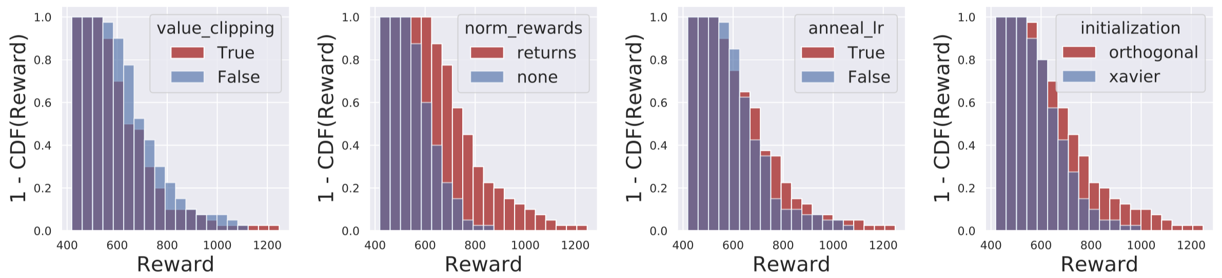
The results of this ablation study are clear: these additional optimizations have a profound effect on PPO’s performance.
So, what is going on? If these optimizations matter so much, to what extent can PPO’s success be attributed to the principles of the framework that this algorithm was derived from?
To address this questions, in our next post, we’ll start looking at the tenets of this policy gradient framework, and how exactly they are reflected in deep policy gradient algorithms.