Deep learning models often exhibit consistent patterns of errors. These errors tend to correspond to hard subpopulations in the data they are deployed on. How can we go about detecting such hard subpopulations, and moreover doing so at scale? Our recent paper is motivated by this very aim, and presents a framework for automatic distillation and surfacing of a model’s failure modes.
Despite the success of deep learning models at a wide range of classification tasks, they are prone to failing—often by underperforming on “hard” subpopulations corresponding to inputs that were consistently mislabelled, corrupted, or simply underrepresented in the training set. This problem is exacerbated when, as is often the case in practice, deployment conditions deviate from the training distribution. In these cases, the model may have learned (spurious) correlations on the training set that are not predictive on the distribution it is deployed on.
To make this more concrete, consider the task of predicting age (old vs young) based on the CelebA dataset of celebrity face images. It turns out that in this dataset, young women and old men are overrepresented, and thus a model trained on CelebA is likely to leverage the resulting correlation between age and gender in its predictions. Of course, as this correlation does not hold at large, this model would then struggle on inputs representing old women and young men.
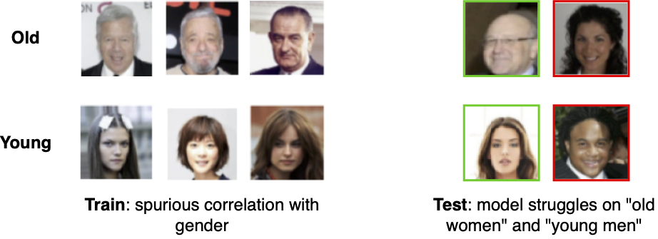
How could we go about identifying these types of model errors? Specifically, for this case, how might we identify that it is the spurious age-gender correlation that is driving these failures?
One option is to manually examine either the dataset or the model itself to identify specific failure modes. Such approaches, however, can be quite labor-intensive, and thus are difficult to scale. Alternatively, one can try to automatically identify and intervene on hard training examples, such as by directly upweighting inputs that were misclassified early in training or training a second model to adversarially identify misclassified instances. However, these approaches also do not fully hit the mark. Specifically, they are not designed to elicit simple, human-interpretable patterns that underlie hard subpopulations (even when these exist). Thus, while such methods are automatic (and certainly scalable), they do not necessarily translate into the type of understanding needed to remedy the underlying data problem.
The framework developed in our recent work intends to bridge this gap between scalability and interpretability. In particular, it enables us to surface subpopulations of hard examples with respect to a given model in a way that is not only automatic, but also naturally suggests an intervention meant to fix them.
Capturing Failure Modes as Latent Space Directions
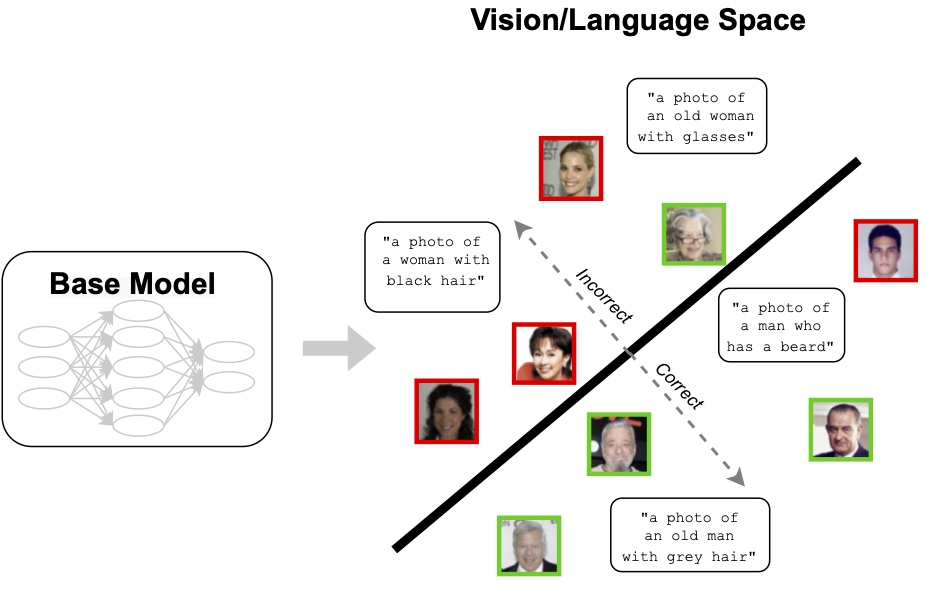
At a high level, our approach aims to model failure modes as directions within a latent space. In the context of the CelebA example we described above, this would correspond to identifying a (separate) direction for each class (old/young) such that the easier examples (“old man”/”young women”) lie in one direction, and the harder examples (“old women”/”young man”) lie in the opposite one. As a result, each such direction would end up capturing the axis of the specific failure mode (here, gender) that the model struggles with.
But how can we learn such a direction to begin with? The key intuition is that, whenever the pattern of errors we aim to capture corresponds to a global failure mode, such as a spurious correlation, the model will make these errors consistently. In other words, the incorrectly classified inputs will share features. As a result, we can capture the pattern behind these mistakes by training a classifier on the feature embedding, which predicts when the model is likely to make an error on a given input.
More specifically, in our framework we train for each class (using a held-out validation set) a linear support vector machine (SVM) that predicts the errors of the original model. The decision boundary of this SVM then establishes a hyperplane separating the correct from the incorrect examples. Moreover, the vector orthogonal to this decision boundary (the normal vector of the hyperplane) represents the direction of the captured failure mode that we are seeking. Indeed, the more aligned an example is with the identified direction, the harder (or easier) the example was for the original model—this is exactly what we needed!
Of course, to make sure this trained SVM can indeed capture the features shared by the errors, we need a suitable featurization for the inputs. In our (image) context, we use CLIP, which embeds both vision and language together using contrastive learning. (As we will see below, using this embedding space has the added benefit of enabling us to automatically caption the captured failure modes, too!)
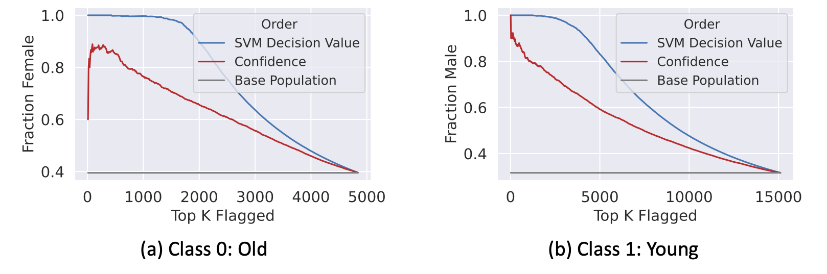
Identifying the gender spurious correlation in CelebA: Let’s return to our example of identifying age for CelebA faces in the presence of a spurious correlation with gender, and apply our framework as described above. The plot below depicts the fraction of test images within each class that are of the minority gender when ordering the images by either their SVM decision value, or by our baseline of using the model’s confidences. We can see that the SVM directions indeed capture the gender-age spurious association, as intended.
Interpreting the extracted failure mode
Now that we’ve distilled the model’s failure modes as directions within the latent space, how can we understand what these failure modes entail exactly?
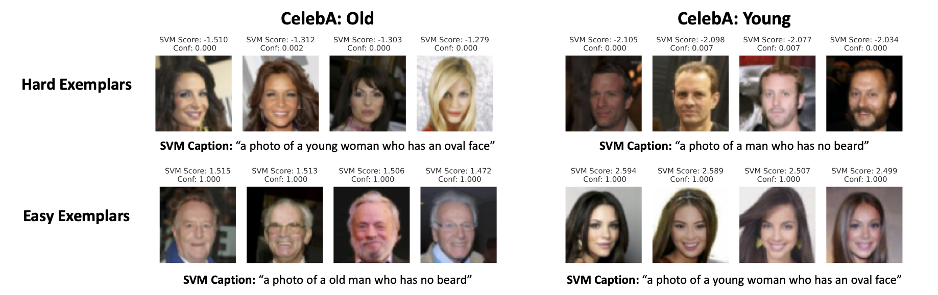
Most Aligned Examples. One approach is to simply surface the examples whose normalized embeddings are most aligned (or anti-aligned) with the extracted direction. These are the images with the most positive or negative SVM decision value (which is proportional to the signed distance from the decision boundary). In doing so, we surface the prototypical examples representing the “most correct” and “most incorrect” examples.
Automatic Captioning. We can, however, go one step further by automatically captioning the extracted failure mode, leveraging the fact that the SVM was trained on a shared vision/language embedding space. Recall that CLIP embeds both images and language into the same latent space. Thus, just as we surfaced the most aligned images above, we can surface the most aligned captions (from some pre-specified set of captions) whose normalized text embedding matches the extracted direction. More details can be found in our paper.
Both techniques are shown below on our running CelebA example. As we can see, images farthest from the SVM decision boundary indeed exemplify the hardest (“old woman”) or the easiest (“old man”) examples. The captions also reflect the corresponding categories.
Man with a Fish: Discovering Failure Modes in the ImageNet Dataset
In the CelebA example we were considering so far, the dataset contained a known, planted spurious correlation (i.e., gender). How will our framework fare when this is not necessarily the case? To study this, let’s apply our framework to the ImageNet dataset (and see our paper for more examples).
What does our framework flag? A broad range of interpretable failure modes—from color biases (e.g., the model struggles on red wolves with white winter coats) to reliance on co-occurring objects (e.g., the model more easily classifies the tench fish in the presence of a person).
Are the flagged subpopulations actually challenging for the original model? To check this, we would ideally compare the difference in test accuracy between the “easy” and “hard” subpopulations proposed by our framework. For example, in the above example of the tench fish, we would hope that tenches described by the “easy” caption (“a photo of an orange fish with a person”) have a higher accuracy on held-out examples than those described by the “hard” caption (“a photo of a close-up fish”).
However, we do not have annotations for the sub-groups of ImageNet necessary to execute this measurement directly. Still, as a proxy, we can use the CLIP shared vision/language embedding space to approximate these sub-group accuracies. So, for example, to evaluate the model’s performance on people with orange fish, we simply check its accuracy on the images whose CLIP embeddings are closest (in cosine distance) to the embedded SVM caption “a photo of an orange fish with a person”.
Performing this kind of evaluation for all the 1000 of ImageNet classes, we find that the original model’s accuracy on the images closest to the “hard caption” is consistently (and significantly) lower than those closest to the “easy caption.” In other words, our framework successfully surfaces the patterns of failure modes. Furthermore, as we describe in the paper, these surfaced patterns guide effective interventions too.
Conclusion
In this post, we introduced a framework for automatically identifying and captioning coherent subpopulations that are especially hard, or easy, for a given model to classify. In particular, our framework harnesses (linear) classifiers to distill the model’s failure modes as meaningful directions in the latent space. Our framework was able to surface challenging subpopulations in widely used datasets such as ImageNet: check out our paper for even more examples (and datasets)!
Overall, we view our methodology as a first step toward building a toolkit for scalable dataset exploration and debiasing—we believe, however, that there is much more to do. For example, we consider only relatively straightforward data interventions (such as upweighting and filtering). Can we come up with more sophisticated interventions to improve the model’s performance on the identified subpopulations? In particular, given all the recent enormous progress on text-to-image generation, one especially promising approach to explore here could be to generate new data that is tailored to the model’s weaknesses (for example, by using DALL-E 2 or ImageGen).