How does the internal computation of an ML model transform inputs into predictions?
Consider a standard ResNet50 model trained on an image classification task. Is it possible to understand how the convolution filters in this model transform an input image to its predicted label? Or, how the attention heads in GPT-3 contribute to next-token predictions? Grasping how these model components—architectural “building blocks” such as filters or heads—collectively shape model behavior (including model failures) is difficult. After all, deep networks are largely black-boxes—complex computation graphs with highly non-linear interactions among model components.
Motivated by this challenge, a line of work in interpretability aims to shed light on internal model computation by characterizing the functionality of individual components, e.g., curve detectors and object-specific filters in vision models, or knowledge neurons and induction heads in language models. The approaches developed as part of this line of work aim to “zoom in” on specific model behaviors and/or components in a variety of ways.
In our recent paper, we take a different, complementary perspective. Instead of “zooming in” on individual components, we study how model components collectively combine to yield model predictions. Specifically, we ask:
How do changes to model components collectively change individual predictions?
Explicitly Modeling Model Computation
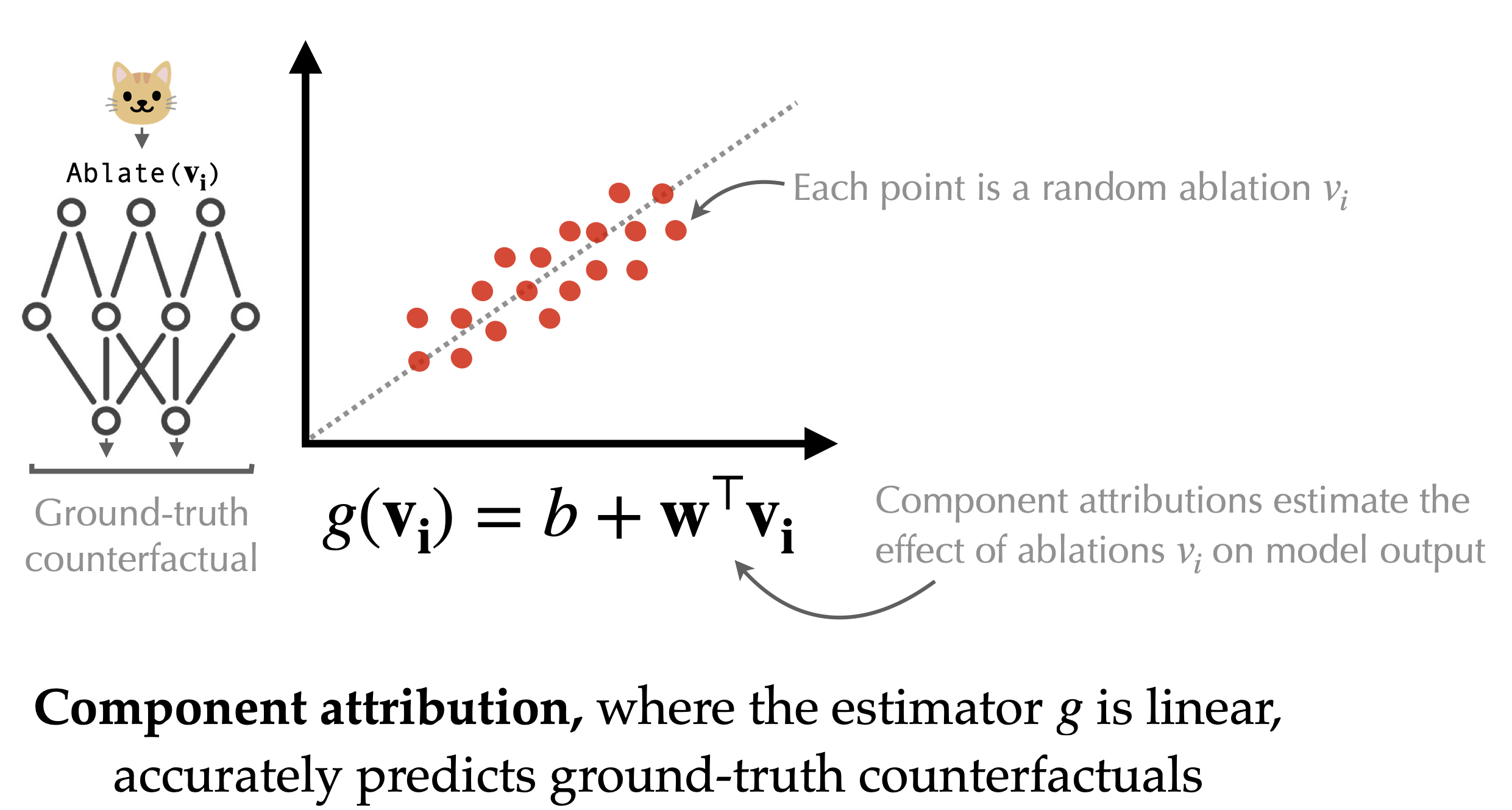
To tackle the question above, we introduce a task called component modeling. The goal of component modeling is to build a simple and interpretable estimator of how a model’s output would change in response to interventions, or ablations, made to its components. Intuitively, the key idea here (illustrated in the figure below) is that if we truly understood how model components contribute to a prediction, we should be able to estimate how the prediction would change if we were to change some components:

Our paper focuses on a special “linear” case of component modeling, which we call component attribution. As shown below, a component attribution for a given model prediction first assigns a score to each model component, and then estimates the counterfactual effect of ablating a set of components as the sum of their corresponding scores:

Component attributions are simple—they decompose a given prediction into additive contributions from each model component. They are also interpretable, in that the “score” assigned to a component signifies the “contribution” of that component to the prediction of interest (while abstracting away the complexity of the model’s internal computation).
Aside: We’ve explored a similar line of thinking—understanding via prediction—in our work on datamodeling, where the goal is to predict model behavior as a function of training data. Component models and component attribution can be seen as analogs of datamodels and data attribution (or linear datamodeling) in “component space,” rather than “training dataset space.”
Estimating Co mponent A ttributions via R egression (COAR)
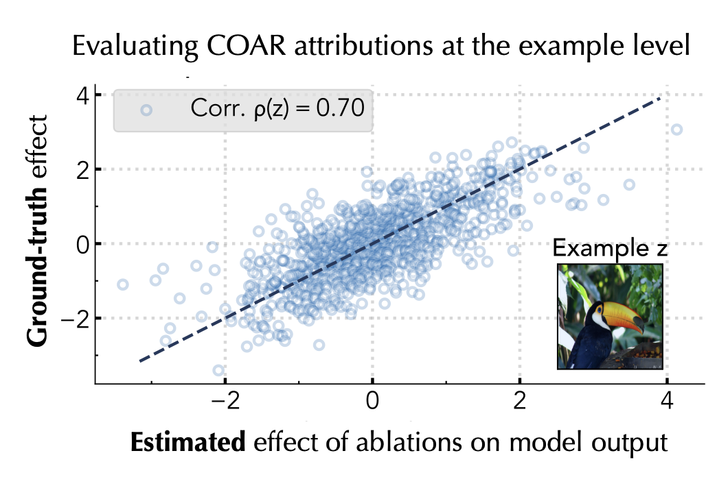
A priori, it’s unclear whether component attributions are expressive enough to capture the (inherently non-linear) map from components to predictions in deep networks. However, we find that on vision models (e.g., ImageNet ViTs) and language models (e.g., Phi-2) one can actually compute accurate component attribution—that is, linearity suffices to predict the effect of component ablations (!), as shown below:

To compute these attributions (i.e., the coefficient vector \(w\) above), we propose a simple method—called COAR (Component Attribution via Regression)—that turns this task into a standard supervised learning problem, and solves it in two steps:
- Construct a dataset of component ablations. We randomly ablate random subsets of components and record both the ablation itself, as well as how the model’s output changes for each example of interest. This gives us a dataset of component ablations and their corresponding effects on the model predictions.
- Fit a linear regression model. We fit a linear model that takes as input an “ablation vector” (a binary vector that encodes the ablated components) and predicts the ablation effect on a given example’s prediction. The learned weights of this linear model serve as our component attributions, quantifying the contribution of each component to the model’s prediction.
That’s it! Both steps of our component attribution method, COAR, are scalable and general, i.e., completely agnostic to model architecture. This allows us to stress-test the effectiveness of COAR attributions in a systematic manner.
Are COAR attributions accurate?
Let’s come back to our ResNet-50, trained on the ImageNet dataset. We’ll view this model as a composition of 22,720 components, each corresponding to a convolutional filter. Can we use COAR to predict how this model will respond to component ablations (in this case, ablation corresponds to zeroing out the parameters of a given set of filters)?
To answer this question, we use COAR to estimate component attribution for each of the 50,000 examples in the ImageNet validation set. The result is a set of 50,000 component attributions–each attribution estimating how every component contributes to the model’s prediction on the corresponding ImageNet example.
To see whether the resulting attributions are indeed valid, we simply check whether component attributions accurately estimate the effect of (randomly) ablating random subsets of components on model outputs.

For example, the figure above focuses on a single ImageNet example. Each dot corresponds to a (random) set of model components. The y value of a given dot is the counterfactual effect of ablating that set of components (i.e., setting the corresponding parameters to zero); the x axis is our estimate of that counterfactual effect, as given by the example’s component attribution. The ground-truth and attribution-estimated effects of (random) component ablations exhibit a high correlation of 0.70, meaning that at least for this example, component attributions are quite good at predicting model behavior!
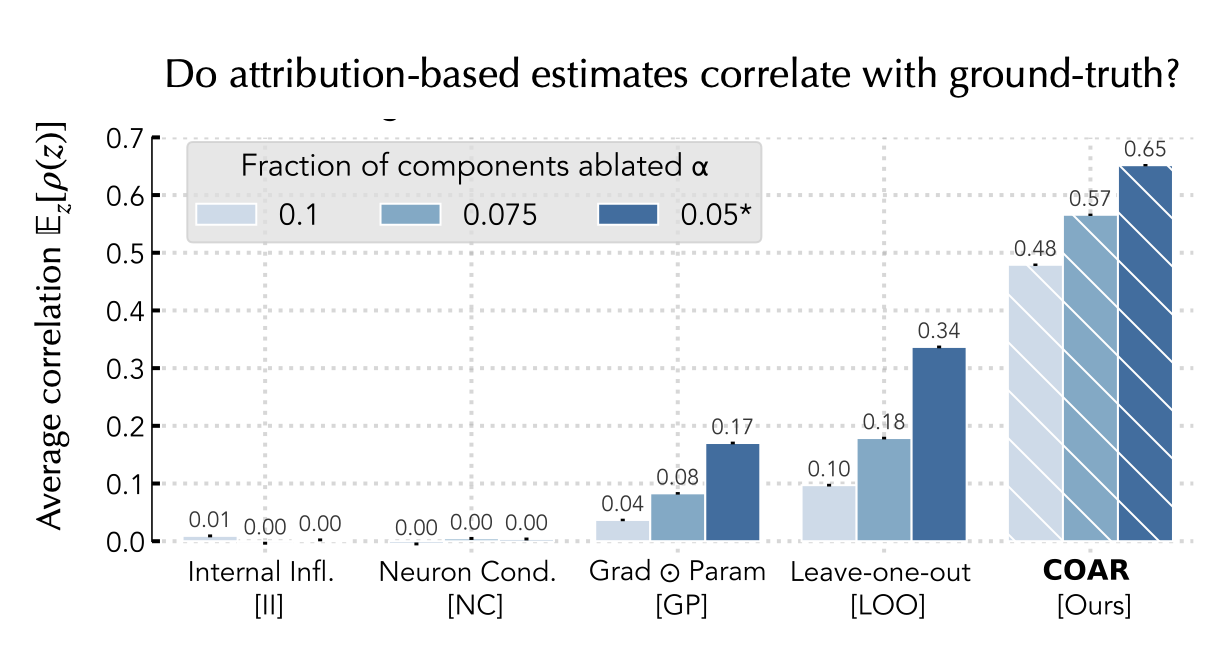
In the figure below, we turn this into an aggregate analysis. That is, we evaluate the average correlation between the ground-truth ablation effects and attribution-based estimates over all validation examples—to test the limits of COAR, we also vary the fractions of components ablated and study how COAR’s performance changes. As baselines, we adapt several notions of “component importance” (some used by prior work, and some that we designed ourselves) to the component attribution setting:

Overall, we find that COAR consistently outperforms multiple attribution baselines by a large margin across datasets and models.
For a more thorough evaluation of COAR attributions, check out our paper. We stress-test there the predictive power of COAR attributions on several other model architectures (e.g., CLIP ViTs, Phi-2, and even simple MLPs) and tasks (e.g., next-token prediction and zero-shot classification).
Up next: applications
What can we actually do with these component attributions? Do they have any practical utility? In our second post, we’ll explore how COAR attributions enable effective model editing. Specifically, we will dive there into the connection between attribution and model editing, and apply COAR to two editing tasks. Stay tuned!
