In this blog post we use datamodels to identify and study a new form of model brittleness.
Recap: Datamodels
In our last post, we introduced datamodels: a framework for studying how models use training data to make predictions. While we summarize datamodels in short below, if you haven’t yet read about datamodels we recommend reading our last post for the full picture.
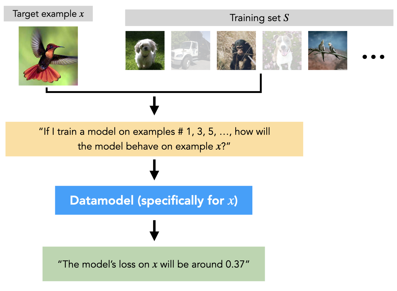
Consider a training set $S$ (e.g., a set of images and labels from a computer vision dataset), a learning algorithm $\mathcal{A}$ (e.g., training a deep neural network from scratch with SGD), and a target example $x$ (e.g., a test image and label from the same dataset). A datamodel for the target example $x$ is a parameterized function that takes as input a subset $S’$ of the original training set $S$, and predicts the outcome of training a model on $S’$ (using $\mathcal{A}$) and evaluating on $x$. In other words, a datamodel predicts how the choice of a specific training subset changes the final model prediction.
Our last post focused on constructing linear datamodels (one for each CIFAR-10 test image) that accurately predict the outcome of training a deep neural network from scratch on subsets of the CIFAR-10 training set.
Today, we’ll use datamodels to investigate deep neural networks’ predictions. Specifically, we’ll introduce and measure data-level brittleness: how sensitive are model predictions to removing a small number of training set points?
Data-level brittleness: a motivating example
Consider this image of a boat from the CIFAR-10 test set:

A deep neural network (ResNet-9) trained on CIFAR-10 correctly classifies this example as a boat with 71% (softmax) confidence. The classification is also “robust” in the sense that over different training runs (each with a different random initialization of the network, batch ordering, data augmentation, etc.), the trained model classifies this example correctly 84% of the time.
It turns out, however, that if we remove just the following nine images from the CIFAR-10 training set…

…models trained with the exact same training procedure (applied to the remaining 49,991 images in the training set) correctly classify the boat only 35% of the time! Furthermore, when we remove only 11 additional training images, the probability of correct classification decreases to merely 10% (the accuracy of a random classifier!).
Model behavior on this boat image exemplifies data-level brittleness. Models confidently and consistently output correct predictions, but these predictions hinge on a very small set of training examples. (One might hypothesize that in this case, brittleness stems from the fact that there are very few training examples of boats on land or grass.)
Quantifying brittleness with datamodels
How do we actually measure data-level brittleness? In the example above, models misclassified the boat after we removed nine images. These were nine specifically chosen images, however: removing nine randomly chosen training images of boats does not at all degrade models’ probability of correctly classifying the boat image. Even removing the nine most similar training examples to the boat image (e.g., in terms of representation space distance) degrades this probability by only 4%.
So, how do we find the “right” images to remove? Specifically, what we’re looking for is the smallest subset of the training set whose removal induces misclassification on average, i.e.,
\begin{align} \tag{1} \label{eq:origobj} \min_{R \subset S} |R’|, \text{ such that }\mathbb{E}[\text{margin of a model trained on } S \setminus R \text{ on } x] \leq 0. \end{align}
Unfortunately, problems like this (optimizing a black-box function over the space of all possible subsets of a large set) are computationally challenging to solve. In the worst case, to find the smallest set satisfying the above condition we would have to train several models for each possible training subset.
This is where datamodels come in. Recall that for a target example $x$ (e.g., our boat example from before), we can construct (read our previous post to see how) a datamodel $g$ that, for any subset of the training set $S’$, returns an estimate:
\begin{align} g(S’) \approx \mathbb{E}[\text{margin of a classifier trained on $S’$ when evaluated on $x$}]. \end{align}
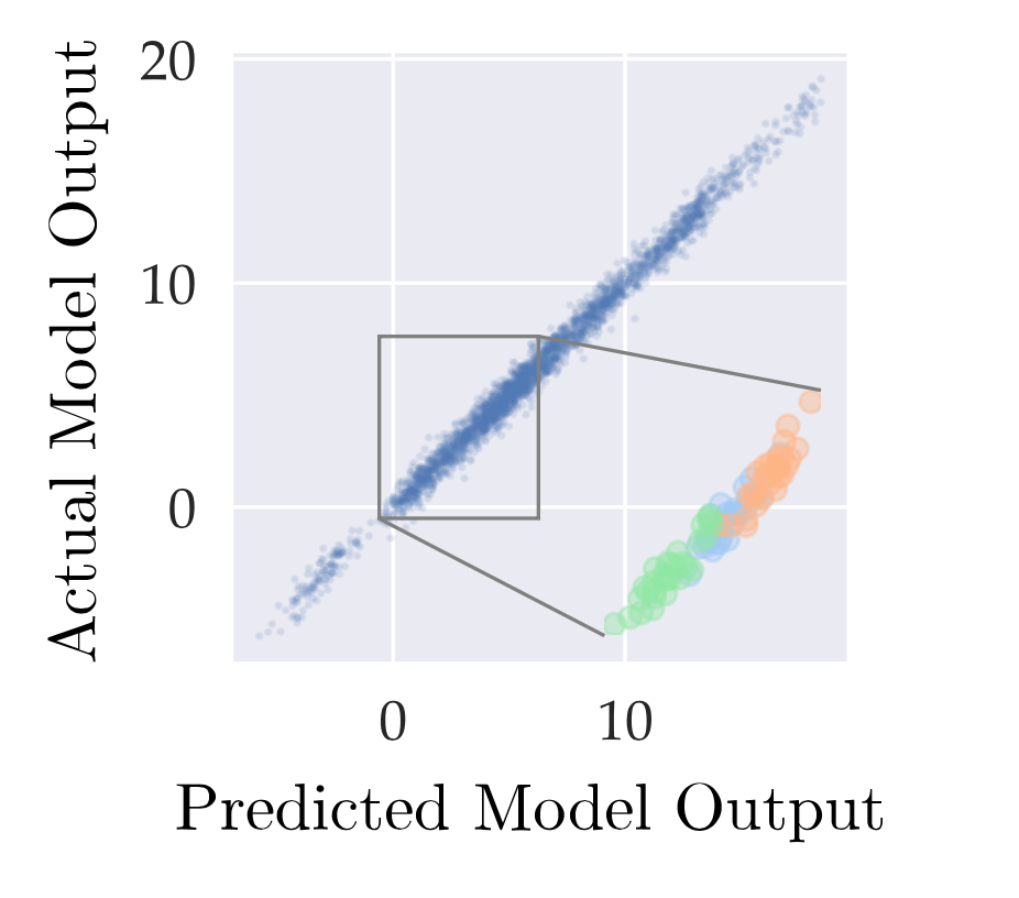
(Here, the expectation is taken over training non-determinism.) Datamodel estimates can be highly accurate. For example, see the following graph of predicted average margin $g(S’)$ against true average margin (the RHS above) from our last post:
Datamodel predictiveness means we can (approximately) solve our earlier optimization problem (\eqref{eq:origobj}) by optimizing instead the surrogate objective:
\begin{align} \tag{2} \label{eq:surrogate1} \min_{R \subset S} \vert R \vert \text{ such that } g(S \backslash R) \leq 0 \end{align}
Since $g(\cdot)$ is a simple (linear) function (see the drop-down below for more details), this new optimization problem is computationally easy to solve (and doesn’t involve training additional models).
After finding a subset $R$ that minimizes the surrogate objective above, we can verify that $R$ is an upper bound on the objective above by training a collection of models on the remaining training images $S \setminus R$, and checking to see that the target example is misclassified on average. We can ensure we actually get an upper bound on the size of the minimum $R$ by solving
\begin{align} \min_{R \subset S} \vert R \vert \text{ such that } g(S \setminus R) \leq C, \end{align}
where $C<0$ is a threshold that we (very coarsely) search for using the verification procedure—if the image isn’t misclassified on average, we can decrease $C$.
Looking at brittleness in aggregate
So far in this post, we’ve seen an example of data-level brittleness, and provided a datamodel-based method for estimating the brittleness of any given prediction. How brittle are model predictions as a whole?
We use our datamodel-based approach to estimate the data-level brittleness of each image in (a random sample of) the CIFAR-10 test set. Specifically, for each test image, we estimate (and bound) the number of training images one would need to remove in order to flip models’ predictions on the test image. We plot the cumulative distribution of these estimates below: a point $(x, y)$ on the blue line below indicates that a $y$ fraction of test set predictions are brittle to the removal of at most $x$ training images.

It turns out that our motivating boat example is not so unusual. In fact, for around 20% of the CIFAR-10 test images it suffices to remove fewer than 60 training images to induce misclassification! Also, for around half of the test examples, it suffices to remove fewer than 250 training images (still only 0.5% of the training set).
The other lines in the graph above illustrate just how hard it is to identify prediction brittleness via other means. Each one represents a different heuristic: a point $(x, y)$ on the line indicates that for a $y$-fraction of the test set, removing the $x$ most similar images to the target example (according to the corresponding heuristic) is necessary to flip models’ predictions. (See Appendix F.2 in our paper for more details on these baselines!)
Bonus: Label-flipping attacks
One immediate consequence of the techniques we discovered in this blog post is the existence of strong label-flipping attacks. So far, we’ve looked exclusively at the result of removing training images—if we use the exact same technique but instead just flip the labels of the images we would have removed, we find more severe brittleness:

The dashed line above is the same as the blue line from earlier—the new solid blue line shows that for over half of the CIFAR-10 test images, we are able to induce misclassification by relabeling just 35 (target-specific) images!
Conclusion
In this post, we introduced a new notion of model brittleness, examined how to quantify it with datamodels, and demonstrated that a large fraction of predictions on the CIFAR-10 test set are quite brittle.
Our results demonstrate one of many ways in which datamodels can be a useful proxy for end-to-end training. More broadly (and as we’ll see in our upcoming posts!), datamodels open the door to many other fine-grained analyses of model predictions.