“Missingness”, or the absence of features from an input, is a concept that is fundamental to many model debugging tools. In our latest paper, we examine the challenges of implementing missingness in computer vision. In particular, we demonstrate how current approximations of missingness introduce biases into the debugging process of computer vision models. We then show how a natural implementation of missingness based on VITs can mitigate these biases and lead to more reliable model debugging.
Deep learning models can learn powerful features. However, these learned features can be unintuitive or spurious. Indeed, recent studies have pointed out that ML models often leverage unexpected—and, in fact, undesirable—associations. These include image pathology detection models that rely on pen marks made by radiologist and image classifiers that focus too much on backgrounds or on texture. Such prediction mechanisms can cause models to fail in downstream tasks or new environments.
How can we detect model failures caused by relying on such brittle or undesirable associations? Answering this question is a major goal of model debugging. Work in this context brought forth techniques that allow, for example, surfacing human aligned concepts, probing specific types of bias a model uses, or highlighting features that were important for a specific prediction.
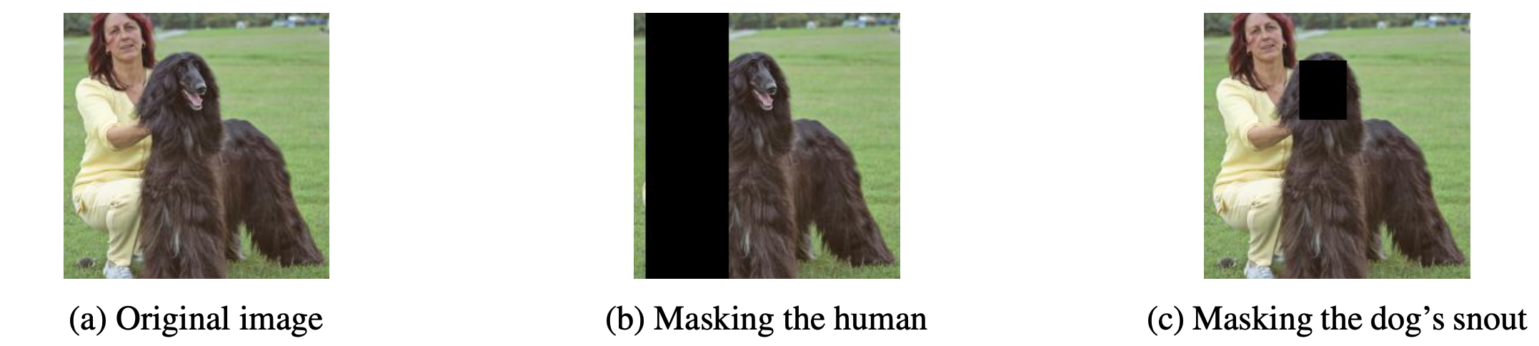
A common theme in many of these debugging methods is to study model behavior on so-called counterfactual inputs, i.e., inputs with and without specific features. For example, consider the image of a dog being held by its owner below. By removing the owner from the image, we can study how much our model’s prediction depends on the presence of a human. In a similar vein, we can remove parts of the dog (head, body, paws) to identify which ones among them are most critical for correctly classifying the image. This concept of “the absence of a feature” from the input is sometimes referred to as missingness.
Indeed, this primitive of missingness is used quite a lot in model debugging techniques. For example, widely-used methods such as LIME and integrated gradients leverage it. It also has been applied to radiology images to understand the regions of the scan that are important for diagnoses, or to flag spurious correlations. Finally, in natural language processing, model designers often remove words to understand their impact on the output.
Challenges of implementing missingness in computer vision
Missingness is a rather intuitive notion: we simply would like the model to predict as if the corresponding part of the input didn’t exist. Also, in a domain such as NLP implementing this primitive is fairly straightforward: we simply drop the corresponding words from the sentence. However, in the context of computer vision, its proper implementation turns out to be much more challenging. This is because images are spatially contiguous objects: it is unclear how to leave a “hole” in the image.
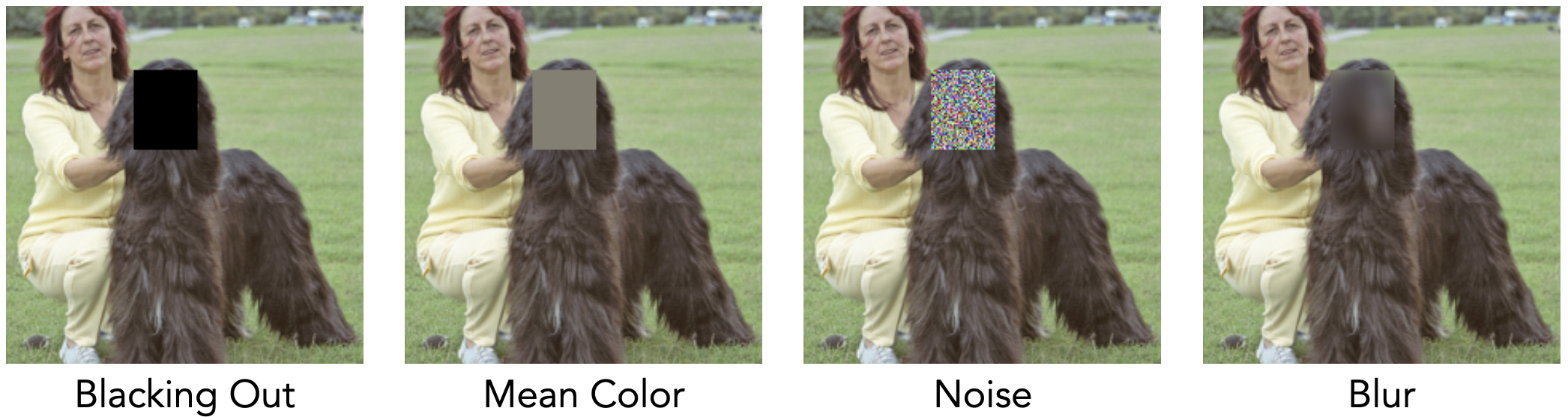
Researchers thus have come up with all kinds of ways to “fill” such hole, i.e., approximating missingness by replacing the region with other pixels. This involves blacking out the pixels, replacing them with random noise, or blurring the corresponding image region. However, these approaches, even though very natural, turn out to have unintended effects. For example, researchers found that saliency maps generated with integrated gradients are quite sensitive to the chosen baseline color of the filling, and thus can change significantly based on the (arbitrary) choice of that missingness approximation.
Missingness approximations can create bias
So, what impact do such missingness approximations actually have on the resulting model predictions? In our recent work, we systematically investigate the bias that these approximations can imbue. Specifically, we find that models end up using masked out regions to make predictions rather than simply ignoring them.
For example, take a look below at the image of a spider from ImageNet, where we have removed various regions from the image by blacking out the corresponding pixels.
It turns out that irrespective of what subregions of the image are removed, a standard CNN (e.g., ResNet-50) outputs incorrect classes, even when most of the foreground object is not obscured. In fact, taking a closer look at the randomly masked images, we find that the model seems to be relying on the masking pattern itself to make the prediction (e.g., predicting class “crossword”).
To analyze this bias more quantitatively, we measure how missingness approximations impact the output class distribution of a Resnet-50 classifier (over the whole dataset). Specifically, we iteratively black out parts of ImageNet images, and keep track of how the probability of predicting any one class changes. Before blacking out any pixels, the model predicts a roughly equal number of each class on the ImageNet test set (which is what one would expect given that this test set is class balanced). However, when we apply missingness approximations, this distribution skews heavily toward classes such as maze, crossword puzzle, and carton.
Our paper investigates this missingness bias in more depth by exploring different approximations, datasets, mask sizes, etc.
Missingness bias in model debugging: A case study on LIME
As we mentioned earlier, missingness primitive is often used by model debugging techniques—how does the above-mentioned bias impact them? To answer this question, we focus on a popular feature attribution method: local interpretable model-agnostic explanations, or LIME.
The image above depicts an example LIME explanation generated for a ResNet-50 classifier. Specifically, for a given image, LIME generates a heatmap highlighting the regions of the image based on how much they impact prediction (according to LIME). While sometimes LIME highlights the foreground object (which is what one would expect), in most cases it also highlights rather irrelevant regions scattered all over the image. Why is this the case?
Although we can’t say for sure, we suspect that this behavior is caused in large part by the fact that the underlying ResNet-50 classifier relies on masked regions in the image to make predictions, and this tricks it into believing that these regions are important. In our paper, we perform a more detailed quantitative analysis of the missingness bias in LIME explanations, and find that it indeed makes them more inconsistent and, during evaluation, indistinguishable from random explanations.
A more natural implementation of missingness
What is the right way to represent missing pixels then? Ideally, since replacing pixels with other pixels can lead to missingness bias, we would like to be able to remove these regions altogether. But what about the need of having the images be represented by contiguous inputs?
Certainly, convolutional neural networks (CNNs) require such spatial contiguity because convolutions slide filters across the image. But do we even need to use CNNs? Not really!
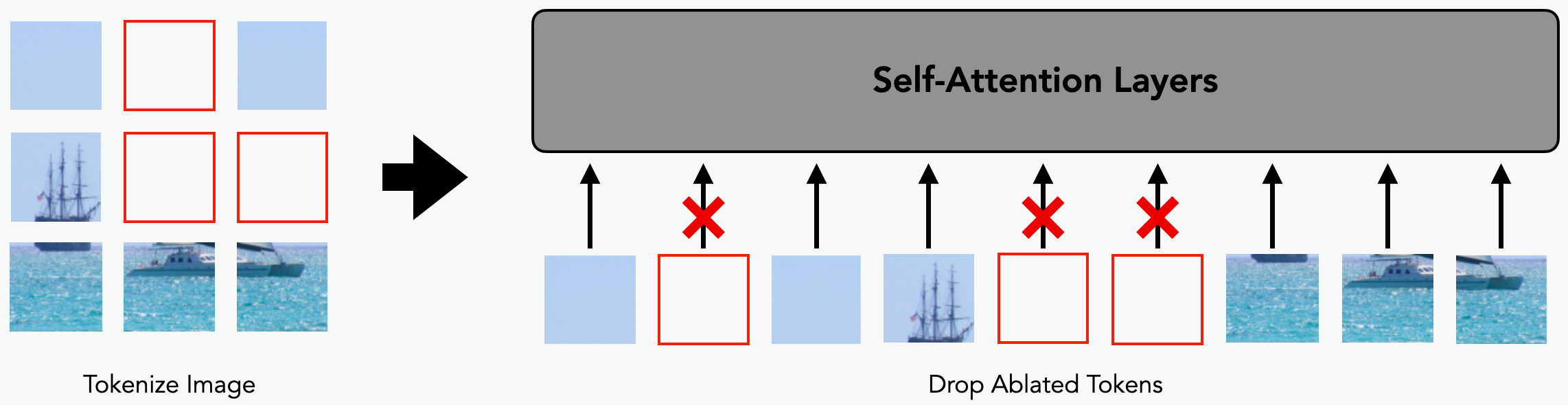
How about we turn to a different architecture: vision transformers (ViTs)? Unlike CNNs, ViTs do not use convolutions and operate instead on sets of patches that correspond to positionally encoded regions of the image. Specifically, a ViT has two stages when processing an input image:
- Tokenization: split the image into square patches, and positionally encode these patches into tokens.
- Self-attention: pass the set of tokens through several self-attention layers.
After tokenization, the self-attention layers operate on the set of tokens rather than the entire image. Thus, ViTs enables a far more natural implementation of missingness: we can simply drop the tokens that encode the region we want to remove!
Mitigating missingness bias through ViTs
As we now demonstrate, using this more natural implementation of missingness turns out to substantially mitigate the missingness bias that we saw earlier. Indeed, recall that, with a ResNet-50, blacking out pixels biased the model toward specific classes (such as crossword). But, a similarly sized ViT-small (ViT-S) architecture is able to side-step this bias (when we implement token dropping), maintaining a correct (or at least related) prediction.
This difference is even more striking when we examine the output class distribution corresponding to removal of image regions: while for our ResNet-50 classifier we have seen this distribution being skewed toward certain classes, for the ViT classifier, this distribution remains close to uniform.
Improving model debugging with ViTs
So, we have seen that ViTs allow us to mitigate missingness bias. Can we thus use ViTs to improve model debugging too? We return to our case study of LIME. As we demonstrated earlier, LIME relies on a notion of missingness, and is thus vulnerable to missingness bias when using approximations like blacking out pixels. What happens when we use ViTs and token dropping instead?
The figure above displays examples of the LIME explanations generated for a ResNet classifier and for a ViT classifier (dropping tokens). Qualitatively, one can see that the explanations for the ViT seem more aligned with human intuition, highlighting the main object instead of regions in the background. We confirm these observations with a more quantitative analysis in our paper.
Conclusion
In this post, we studied how missingness approximations can lead to biases and, in turn, impact the model debugging techniques that leverage them. We also demonstrated how transformer-based architectures can enable a seamless implementation of missingness that allows us to side-step missingness bias and lead to more reliable model debugging.