This two-part series overviews our recent work on constructing deep networks that perform well while, at the same time, being easier to debug. Part 1 (below) describes our toolkit for building such networks and how it can be leveraged in the context of typical language and vision tasks. This toolkit applies the classical primitive of sparse linear classification on top of feature representations derived from deep networks, and includes a custom solver for fitting such sparse linear models at scale. Part 2 outlines a suite of human-in-the-loop experiments that we designed to evaluate the debuggability of such networks. These evaluations demonstrate, in particular, that simply inspecting the sparse final decision layer of these networks can facilitate detection of unintended model behaviours—e.g., spurious correlations and input patterns that cause misclassifications.
As ML models are being increasingly deployed in the real world, a question that jumps to the forefront is: how do we know these models are doing “the right thing”? In particular, how can we be sure that models aren’t relying on brittle or undesirable correlations extracted from the data, which undermines their robustness and reliability?
It turns out that, as things stand today, we often can’t. In fact, numerous recent studies have pointed out that seemingly accurate ML models base their predictions on data patterns that are unintuitive or unexpected, leading to a variety of downstream failures. For instance, in a previous post we discussed how adversarial examples arise because models make decisions based on imperceptible features in the data. There are many other examples of this—e.g., image pathology detection models relying on pen marks made by radiologists; and toxic comment classification systems being disproportionately sensitive to identity-group related keywords.
These examples highlight a growing need for model debugging tools: techniques which can facilitate the semi-automatic discovery of such failure modes. In fact, a closely related problem of interpretability—i.e., the task of precisely characterizing how and why models make their decisions, is already a major focus of the ML community.
How to debug your deep network?
A natural approach to model debugging is to inspect the model directly. While this may be feasible in certain settings (e.g., for small linear classifiers or decision trees), it quickly becomes infeasible as we move towards large, complex models such as deep networks. To work around such scale issues, current approaches (spearheaded in the context of interpretability) attempt to understand model behavior in a somewhat localized or decomposed manner. In particular, there exist two prominent families of deep network interpretability methods—one that attempts to explain what individual neurons do [Yosinski et al. 2015, Bau et al. 2018] and the other one aiming to discern how the model makes decisions for specific inputs [Simonyan et al. 2013, Ribeiro et al. 2016]. The challenge however is that, as shown in recent studies [Adebayo et al., 2018, Adebayo et al., 2020, Leavitt & Morcos, 2020], such localized interpretations can be hard to aggregate, are easily fooled, and overall, may not give a clear picture of the model’s reasoning process.
Our work thus takes an alternative approach. First, instead of trying to directly obtain a complete characterization of how and why a deep network makes its decision (which is the goal in interpretability research), we focus on the more actionable problem of debugging unintended model behaviors. Second, instead of attempting to grapple with the challenge of analyzing these networks in a purely “post hoc” manner, we train them to make them inherently more debuggable.
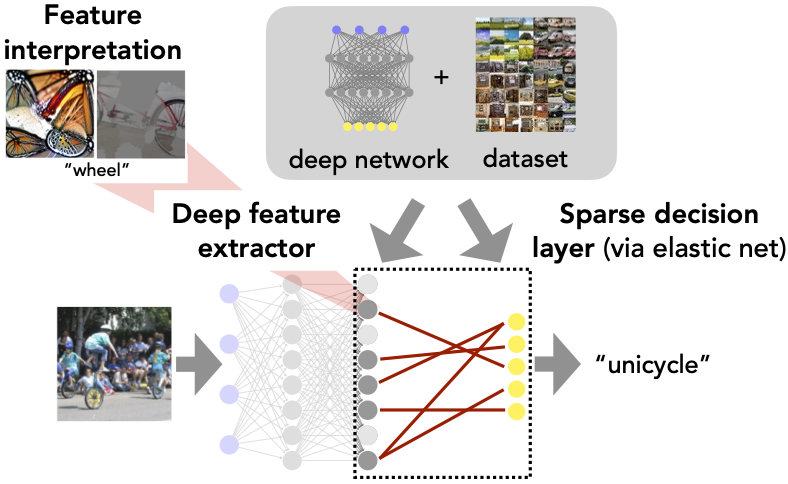
The specific way we accomplish this goal is motivated by a natural view of a deep network as a composition of a feature extractor and a linear decision layer (see the figure below). From this viewpoint, we can break down the problem of inspecting and understanding a deep network into two subproblems: (1) interpreting the deep features (also known in the literature as neurons—that we will refer to as features henceforth) and (2) understanding how these features are aggregated in the (final) linear decision layer to make predictions.
Let us now discuss both of these subproblems in more detail.
Task 1: Interpreting (deep) features
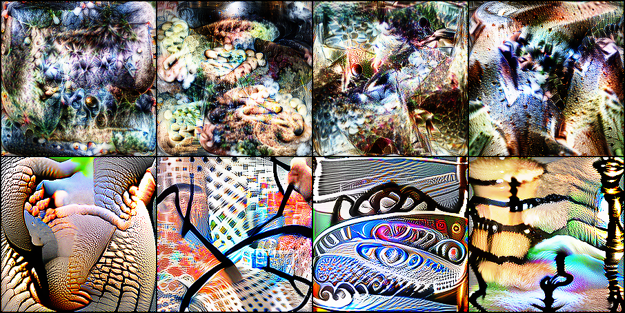
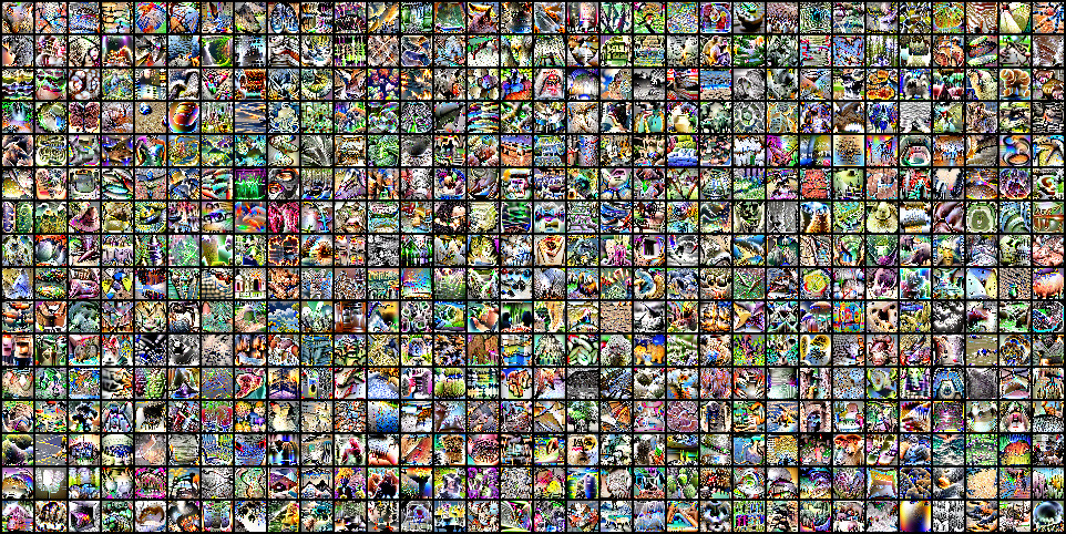
Given the architectural complexity of deep networks, precisely characterizing the role of even a single neuron (in any layer) is challenging. However, research in ML interpretability has brought us a number of heuristics geared towards identifying the input patterns that cause specific neurons (or features) to activate. Thus, for the first task, we leverage some of these existing feature interpretation techniques—specifically, feature visualization, in case of vision models [Nguyen et al. 2019] and LIME, in case of vision/language models [Ribeiro et al. 2016]. While these methods have certain limitations, they turn out to be surprisingly effective for model debugging within our framework. Also, note that our approach is fairly modular, and we can substitute these methods with any other/better variants.
Task 2: Examining the decision layer
At first glance, the task of making sense of the decision layer of a deep network appears trivial. Indeed, this layer is linear and interpreting a linear model is a routine task in statistical analysis. However, this intuition is deceptive—the decision layers of modern deep networks often contain upwards of thousands of (deep) features and millions of parameters—making human inspection intractable.
So what can we do about this?
Recall that the major roadblock here is the size of the decision layer. What if we just constrained ourselves only to the “important” weights/features within this layer though? Would that allow us to understand the model?
To test this, we focus our attention on the features that are assigned large weights (in terms of magnitude) by the decision layer. (Note that all the features are standardized to have zero mean and unit variance to make such a weight comparison more meaningful.)
In the figure below, we evaluate the performance of the decision layer when it is restricted to using: (a) only the “important features” or (b) all features but the important ones. The expectation here is that if the important features are to suffice for model debugging, they should at the very least be enough to let the model match its original performance.
As we can see, this is not the case for typical deep networks. Indeed, for all but one task, the top-k features (k is 10 for vision and 5 for language task) are far from sufficient to recover model performance. Further, there seems to be a great deal of redundancy in the standard decision layer—the model can perform quite well even without using any of the seemingly important features. Clearly, inspecting only the highest-weighted features does not seem to be sufficient from a debugging standpoint.
Our solution: retraining with sparsity
To make inspecting the decision layer more tractable for humans and also deal with feature redundancy, we replace that layer entirely. Specifically, rather than finding better heuristics for identifying salient features within the standard (dense) decision layer, we retrain it (on top of the existing feature representations) to be sparse.
To this end, we leverage a classic primitive from statistics: sparse linear classifiers. Concretely, we use the elastic net approach to train regularized linear decision layers on top of the fixed (pre-trained) feature representation.
The elastic net is a popular approach for fitting linear models in statistics, that combines the benefits of both L1 and L2 regularization. Elastic net solvers yield not one but a series of sparse linear models—each with different sparsity/accuracy—based on the strength of regularization. We can then let our application-specific accuracy vs sparsity needs guide our choice of a specific sparse decision layer from this series.
However, when employing this approach to modern deep networks, we hit an obstacle—existing solvers for training regularized linear models simply cannot scale to the number of datapoints and input features that we would typically have in deep learning. To overcome this problem, we develop a custom, efficient solver for fitting regularized generalized linear models at scale. This solver leverages recent advances in variance reduced gradient methods and combines them with path-algorithms from statistics to get fast and stable convergence at ImageNet scales. We won’t go into much detail here, but we point the curious reader to our paper and our standalone PyTorch package (which might be of independent interest) for more information.
To summarize—the elastic net gives us a sparse decision layer that, in turn, enables us to debug the resulting network by applying the existing feature interpretation methods to a now-significantly-reduced number of features (i.e., only the ones used by the sparse decision layer).
What do we gain from sparity?
Now that we have our methodology in place, we can apply it to standard ML tasks and measure the impact of enforcing sparsity of the final decision layer. Specifically, we discuss the results of applying it to ResNet-50 classifiers trained on ImageNet and Places-10 (a 10-class subset of Places365), as well as BERT models trained on the Stanford Sentiment Treebank and Wikipedia toxic comment classification tasks.
Sparsity at the last layer is (almost) free
Needless to say, the usefulness of our method hinges on the degree of sparsity in the decision layer that we can achieve without losing much accuracy. So how far can we turn the sparsity dial? The answer turns out to be: a lot! For instance, the final decision layer of an ImageNet classifier with 2048 features can be reduced by two orders of magnitude, i.e., to use only 20 features per class, at the cost of only 2% test accuracy loss.
In the following demonstration, one can move the slider to the right to increase the density of the final decision layer of a standard ImageNet classifier. And, indeed, with only 2% of weights being non-zero, the model can already essentially match the performance (74%) of a fully dense layer.
A closer look at sparse decision layers
Our key motivation for constructing sparse decision layers was that it enables us to manually examine the (reduced set of) features that a network uses. As we saw above, our modified decision layers rely on substantially fewer features per class—which already significantly aids their inspection by a human. But what if we go one step further and look only at the “important” features of our sparse decision layer, as we tried to do with the dense decision layer earlier?
As we can see below, for models with a sparse decision layer, the top 5-10 important features are necessary and almost sufficient for capturing the model’s performance. That is, (i) accuracy drops to near chance levels (1/number of classes) if the model does not leverage these features and (ii) using these features alone, the model can nearly recover its original performance. This indicates that the sparsity constraint not only reduces the number of features used by the model, but also makes it easier to rank features based on their importance.
Sparse decision layers: an interactive demonstration
In the following interactive demonstration, you can explore a subset of the decision layer of a (robust) ResNet-50 on ImageNet with either a sparse or dense decision layer:
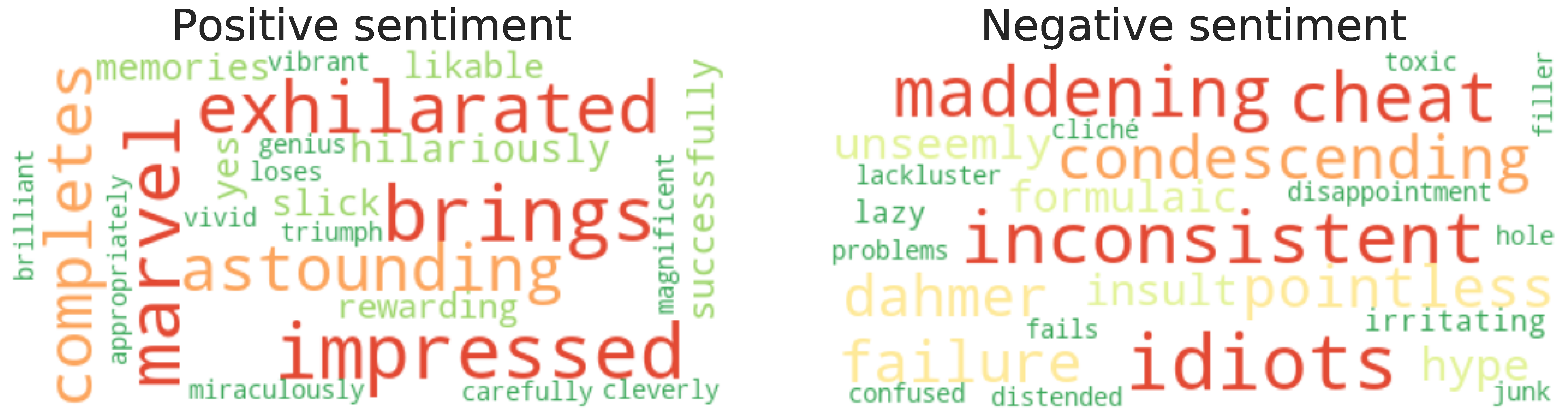
Finally, one should note that the features used by sparse decision layers seem somewhat more human-aligned than the ones used by the standard (dense) decision layers. This observation coupled with our previous ablations studies indicate that sparse decision layers could offer a path towards more debuggable deep networks. But, is this really the case? In our next post, we will evaluate whether models obtained via our methodology are indeed easier for humans to understand, and whether they truly aid the diagnosis of unexpected model behaviors.