ModelDiff: A Framework for Comparing Learning Algorithms

Paper Code
In our recent paper, we introduce a general framework, ModelDiff, for comparing machine learning models trained with two different algorithms. In this post, we illustrate our framework by example, comparing models trained from scratch and models fine-tuned from ImageNet.

Comparing Learning Algorithms

Building ML training pipelines involves many design choices. Even putting the choice of our training dataset aside, we have to decide on a model architecture, an optimization method to train the model, and whether to include one or more regularization techniques. On top of all this, we have to play with a bunch of hyperparameters until we get models that perform well enough on our validation set. This entire pipeline—the aggregate of all train-time design choices—is a learning algorithm, a function mapping training datasets to ML models.

Often, seemingly minor or innocuous tweaks to such a learning algorithm can affect the behavior of the resulting models in subtle and unintended ways. For example, pruning techniques that sparsify models prior to deployment end up hurting performance on underrepresented subpopulations. Random cropping—a standard data augmentation scheme that improves model performance—amplifies texture bias in image classification tasks.

We often want to know how a given design choice modulates the specific features that models learn. To that end, our latest work develops a general framework (called ModelDiff) for performing fine-grained, feature-based comparisons of any two learning algorithms.

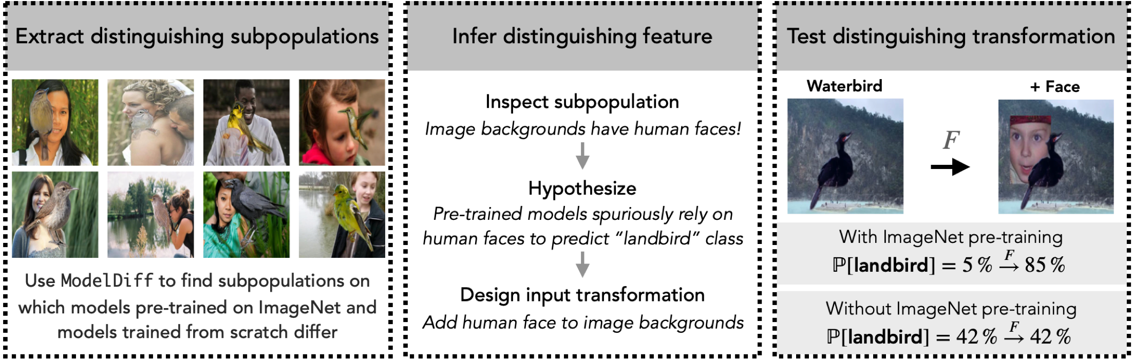
In rest of this post, we will introduce our framework by walking through a specific case study: exploring the effect of ImageNet pre-training on the Waterbirds dataset. In this case study (spoiler alert), we’ll use ModelDiff to find that pre-trained models rely on the presence of a human face in the background to predict “landbird!” Importantly, we’ll do this without having any prior hypotheses, domain knowledge, or dataset annotations.

Case Study: Using ModelDiff to study pre-training

A common design choice in supervised learning is whether to train a model from scratch or fine-tune it from one pre-trained on a larger dataset. (A standard choice for this larger dataset is the ImageNet dataset.)

In this case study, we consider the Waterbirds dataset, for which the task is to classify images of birds overlaid on random backgrounds as either “landbirds” or “waterbirds.” Indeed, on Waterbirds, fine-tuning a pre-trained ImageNet model (rather than training from scratch) significantly improves overall performance.

But is that all pre-training does? In particular, what other (possibly undesirable) impact does pre-training have on the fine-grained behavior of the learned model?

A data-centric perspective

The perspective we adopt in our paper is that models are different insofar as they use different features of the data to make predictions. But how do we know what features models use? This is where our method, ModelDiff, comes in. The core idea behind ModelDiff is that:

Models that use different features to arrive at their final predictions should rely on different training examples to make these predictions.

For instance, suppose we were comparing a texture-biased model to a shape-biased one: when faced with a test example containing a cat in a specific pose, the texture-biased model will rely on cats from the training set with similar texture (e.g., fur), whereas the shape-biased model will rely more on cats in a similar pose.

Below, we translate this intuition into a practical algorithm, applying ModelDiff to our problem of comparing pre-trained models to those trained from scratch:

Step 1: Tracing predictions back to training data with datamodels

To understand which training examples models rely on, we use datamodels—an approach to understanding how instance-wise predictions of (deep) models depend on individual examples in the training dataset $S$. If you’re not familiar with datamodels, we recommend reading our previous posts, or (if you’re in a rush) reading the summary below:

A primer on datamodels (Click to expand)

Linear datamodels. A linear datamodel $\theta_x$ for a test example $x$ is a linear function that takes as input a set of training data indices $S’ \subset [n]$ and predicts the model output on $x$ if we were to train a model on just the corresponding training examples. It turns out that these linear datamodels can surprisingly accurately predict how counterfactual changes to the training dataset change final model predictions! That is, we have that $$\theta_x^\top 1_{S'} \approx \mathbb{E}[\text{margin on $x$ of classifier trained on S’}],$$ where $\mathbf{1}_{S’} \in \{0,1\}^n $ is the indicator vector of $S’$ in the training set $S$. Intuitively, the datamodel weight $(\theta_{x})_i$ signifies the contribution of the $i$-th training example to the model’s performance on test example $x$.

Datamodels as representations. As highlighted in the original paper on datamodels, we can view each linear datamodel $\theta_x$ as a representation (or embedding) of its corresponding test example $x$. It turns out that there are two key properties that arise from this perspective that naturally facilitate comparisons between the corresponding learning algorithms:

Consistent basis: For a fixed training dataset $S$, all linear datamodels share the same basis. That is, coordinate $i$ always corresponds to the importance of the $i$-th training example, regardless of what learning algorithm we use. This conveniently allows for model-agnostic comparisons between learning algorithms that may have entirely different latent representations.
Predictiveness: By design, datamodel vectors are causally predictive of model behavior. Trained models—potentially with different algorithms—that have (distributionally) different outputs on example $x$ end up with dissimilar datamodels for example $x$.

Taken together, these two properties enable a fine-grained analysis of models in terms of how they use training data to make predictions.

The first step in our pipeline is to compute two sets of datamodels $\{\theta^{(1)}_{x_i}: x_i \in T\}$ and $\{\theta^{(2)}_{x_i}: x_i \in T\}$ for the test set $T$, each set corresponding to one learning algorithm. In our case study here, the two sets of datamodels correspond to Waterbirds models trained with and without ImageNet pre-training, respectively.

But before we go ahead, simply visualizing test images and their corresponding “most important training examples” (i.e., those corresponding to the highest datamodel weights) already suggests that models trained with/without ImageNet pre-training are influenced by qualitatively very different training examples:

Step 2: Isolating differences with residual datamodels

The datamodels $\theta^{(1)}_x$ and $\theta^{(2)}_x$ describe how each algorithm uses the training data to make a prediction on a given example $x$. What we’re really interested in, however, are the differences in how these two algorithms use the training data. To isolate these differences, we compute two residual datamodels, $\theta^{(1 \setminus 2)}_x$ and $\theta^{(2 \setminus 1)}_x$ for each example $x$. As illustrated below, the residual datamodel ${\theta}^{(1\setminus 2)}_x$ represents the training direction that influences ImageNet-pretrained models on example $x$ after “projecting away” the component that also influences models trained from scratch:

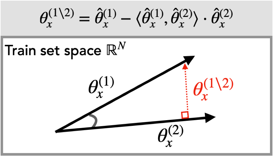
where $\widehat{\theta}_x$ denotes the $\ell_2$-normalized version of datamodel $\theta_x$. Analogously, the residual datamodel $\theta^{(2 \setminus 1)}_x$ encodes a weighted combination of training examples that influence predictions of models trained from scratch but not of models pre-trained on ImageNet.

Step 3: Extracting distinguishing subpopulations with PCA

The outputs of Step 2 above—i.e., the two sets of residual datamodels ${\theta^{(1 \setminus 2)}_i}$ and ${\theta^{(2 \setminus 1)}_i}$—capture how models trained with and without ImageNet pre-training differ, but only at the per-example level. Our goal, however, is to understand global differences in model behavior. To this end, we use principal component analysis (PCA) to distill the residual datamodels into distinguishing training directions, i.e., representative directions in training set space (i.e., in $\mathbb{R}^{n}$) that generally influence predictions of models trained with one algorithm but not the other.

More concretely, we apply PCA to both sets of residual datamodels $\{\theta^{(1 \setminus 2)}_i\}$ and $\{\theta^{(2 \setminus 1)}_i\}$. The output is a set of principal components $v_j \in \mathbb{R}^n$—we can think of each component as a weighted combination of training examples.

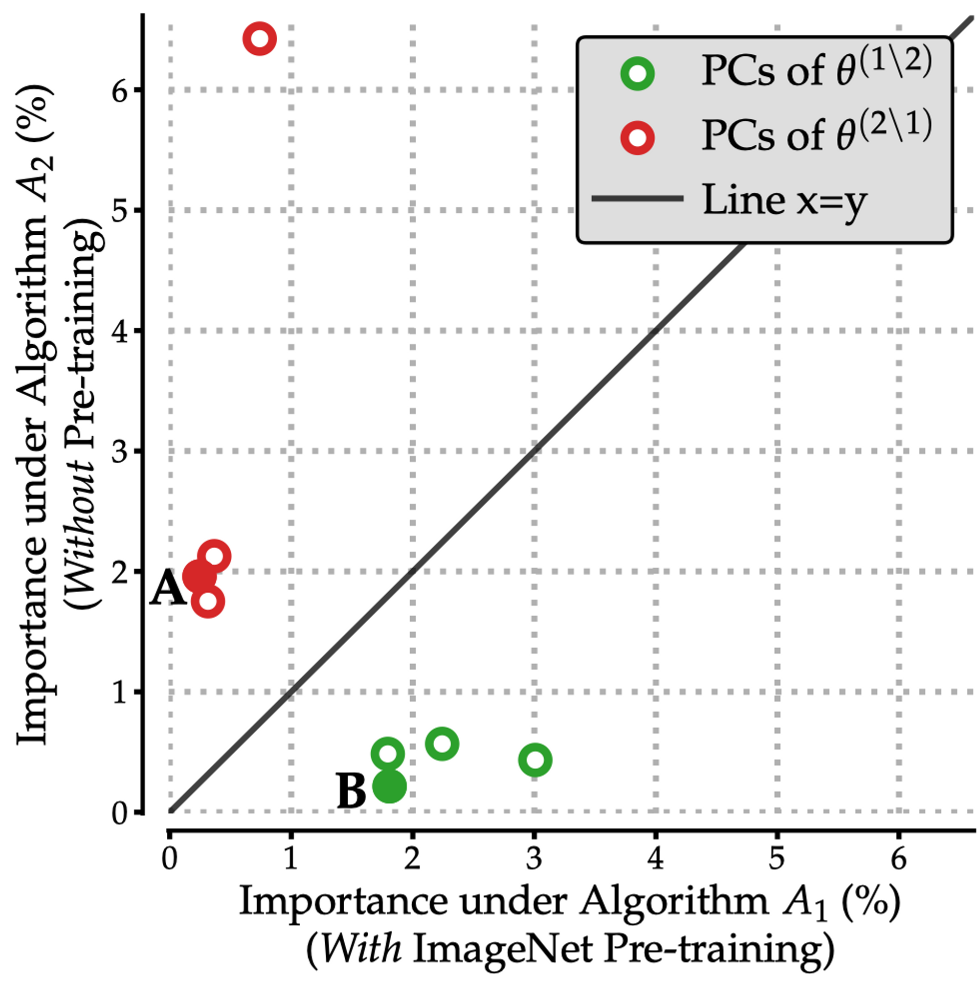
In our paper, we show how to quantify the importance of a given weighted combination of training examples to each algorithm: as shown in the plot below, the top principal components of the residual datamodels $\{\theta^{(1 \setminus 2)}_i\}$ are important to Algorithm 1 (pre-training then fine tuning) but not to Algorithm 2 (training from scratch); and vice-versa for $\{\theta^{(1 \setminus 2)}_i\}$.

Caption: Each red (resp. green) point represent distinguishing training direction—a weighted combination of training examples that influence predictions of models pre-trained on ImageNet significantly more (resp. less) than that of models trained from scratch. The $x$ and $y$ coordinates of each point represent the fraction of explained variance under Algorithm 1 (pre-training) and Algorithm 2 (training from scratch).

We can now take each principal component and look at the test examples whose residual datamodels are most aligned with that direction: this yields a set of subpopulations distinguishing learning Algorithm 1 from 2, and vice versa.

Verifying subpopulations found by ModelDiff

How do we verify though that the distinguishing subpopulations ModelDiff output actually capture meaningful differences in model behavior?

Let’s start by visualizing these subpopulations. That is, let’s take a look at the subpopulations surfaced by distinguishing directions annotated as $\textbf{A}$ and $\textbf{B}$ in the scatterplot above:

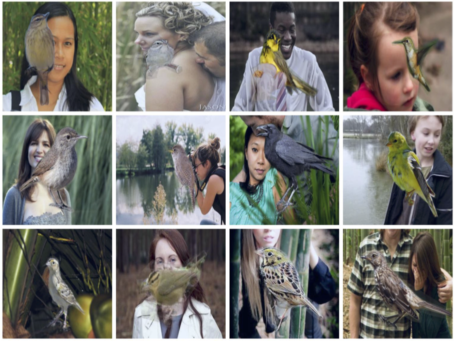
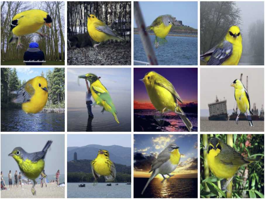
Caption: The subpopulations surfaced by the directions annotated $\textbf{B}$ (left) and $\textbf{A}$ (right) in the scatterplot above. The former has a common feature that is important to pre-trained models but not to from-scratch ones; the latter has a common feature that is important to from-scratch models but not to pre-trained ones.

It seems these surfaced subpopulations indeed highlight semantically meaningful features! For example,

Subpopulation $\textbf{A}$ has images of yellow landbirds or images of yellow blotches in the background. This suggests that models trained from scratch (but not ImageNet-pretrained models) spuriously rely on a “yellow color” feature to predict landbirds.
Subpopulation $\textbf{B}$ surfaces images of landbirds with human faces in the background. This suggests ImageNet-pretrained models finetuned on Waterbirds (but not those trained from scratch) spuriously rely on a “human face” feature to predict landbirds.

Ok, so these are plausible hypotheses, but can we go a step further and actually test whether these inferred features—yellow color and human face—influence model behavior as we suspect they do? Yes, via explicit counterfactual experiments!

Indeed, if ImageNet-pretrained models rely on a “human face” feature, simply adding a face to image backgrounds should consistently change the behavior of these models (but not of models trained from scratch). Similarly, just adding a small yellow patch to images should influence models trained from scratch, but not those that are pre-trained on ImageNet. Is that the case?

It turns out that it is! The plots below demonstrate the effect of adding a yellow patch or a human face on the confidence of models in predicting the class “landbird”.

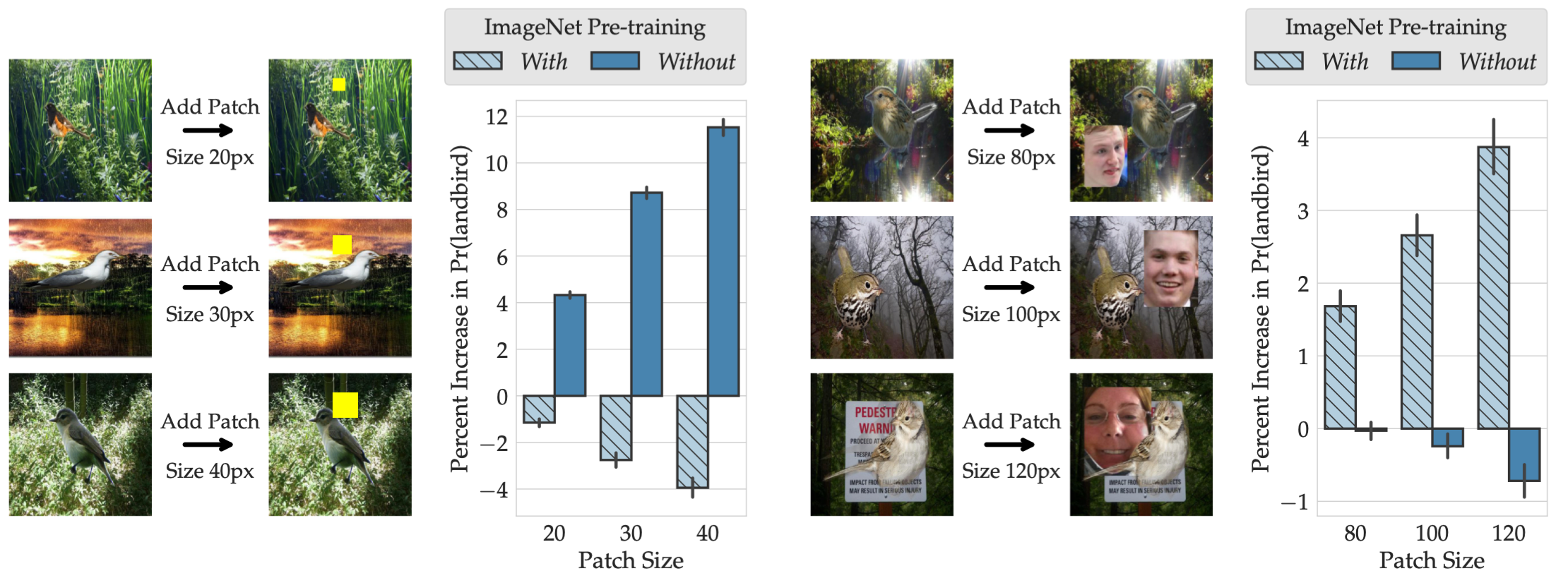
Caption: Treatment effect of distinguishing feature transformations. Adding a yellow square patch to images makes models trained with and without ImageNet pre-training, on average, 9% more and 2% less confident in predicting the label "landbird." On the other hand, adding a human face to image backgrounds makes models trained with and without ImageNet pre-training, on average, 3% and 0% more confident in predicting the label "landbird."

In summary, ModelDiff allowed us to find that ImageNet pre-training significantly reduces dependence on some of the spurious correlations (e.g., yellow color $\rightarrow$ landbird) but also introduces new ones (e.g., human face $\rightarrow$ landbird).

Takeaways

In this post, we introduced a general framework, ModelDiff, for fine-grained, feature-based comparisons of any two learning algorithms. Our framework is general in that we can compare any set of learning algorithms that are applied to a common training set. (For instance, one could even compare a neural network to a random forest classifier.)

In our paper, we further showcase using two other case studies—one on data augmentation and another on SGD hyperparameters—how ModelDiff can help us understand how standard design choices impact model behavior in a fine-grained manner.

More broadly, our framework demonstrates how adopting a data-centric lens and abstracting away internal details of a given model can help us probe properties of learning algorithms.