In our previous post, we discussed the reinforcement learning setup, and introduced the policy gradient—a way of treating reinforcement learning (RL) as an optimization problem.
We also took a closer look at proximal policy optimization (PPO), a popular algorithm based on the policy gradient framework. We discover that PPO tends to employ several optimizations that lie outside of this framework, but have significant impact on performance.
Given these findings, we may want to take another look at our policy gradient framework and ask: to what degree do modern policy gradient algorithms reflect the tenets of this framework?
As a first step towards tackling this question, we want to take a fine-grained look at state-of-the-art deep RL algorithms. In particular, we want to analyze the fundamental primitives which underly them.
In our paper, we considered two prominent deep policy gradient methods: proximal policy optimization (PPO) and trust region policy optimization (TRPO).
We start our investigation with perhaps the most crucial primitive of policy gradient algorithms: gradient estimation.
Gradient estimation
Recall from our last post that policy gradient algorithms work by plugging gradient estimates into a first-order optimization process (like gradient descent). These gradient estimates thus play a critical role in shaping agent performance.
In the policy gradient framework, we estimate gradients by approximating the corresponding expectation with a finite-sample mean. Thus, the quality of gradient estimates is heavily dependent on how this mean concentrates around its expectation. (Note that in the case of PPO and TRPO we don’t use the exact policy gradient that we saw last time, but the variant we do use also boils down to estimating an expectation via finite-sample mean.)
So can we quantify the quality of these estimates? Let us consider the following two experiments.
Gradient variance
In the first experiment, we focus on the gradient variance. Specifically, at iteration \(t\) of training, we measure the gradient variance by first freezing the current policy, and then computing 100 different gradient steps (all with respect to that policy). Next, we measure the average pairwise cosine similarity between the gradient steps. If we are in a regime where gradient variance is quite low, we expect this pairwise similarity to be high. On the other hand, if our gradient estimates are overwhelmed by noise, we expect nearly uncorrelated estimates.
Correlation with the “true” gradient
In the second experiment, we once again start by freezing the agent at some point during training. Then, we use a large number of samples (enough to get a low-variance estimate, as measured by the previous experiment) to estimate the “true” gradient that we want to compute. (While the inability to take infinite samples stops us from obtaining an actual true gradient, we expect this high-sample estimate to be quite close.) We measure the average cosine similarity between the estimated gradient and the aforementioned “true” gradient.
For both these experiments, we train agents to solve the Humanoid-v2 task (a common control benchmark in RL) using both algorithms (PPO, TRPO) with standard training configurations. We freeze agents at several checkpoints during training: 0% (iter. 0/500), 30% (150/500), 60% (300/500), and 90% (450/500). We then plot the two metrics that we defined above (the gradient variance, and correlation with the “true” gradient) as a function of the number of samples used for gradient estimation. Crucially, as is standard, we measure the “number of samples” to be the number of actions the agent takes (not the number of trajectories).
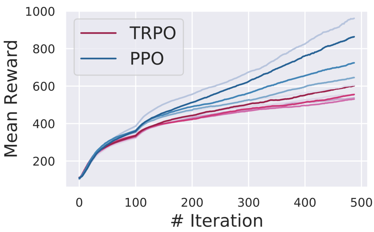
First, we should note that all methods show consistent reward improvement over the entire training process:
Now, we plot below the correlation of the estimates with the “true” gradient:
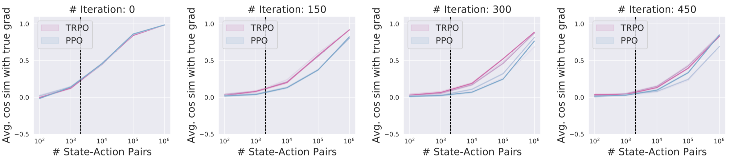
The vertical bar in the graphs above represents the number of samples that we typically use (2000) for gradient estimation when training agents for these benchmarks.
We can see that in the relevant sample regime, the correlation of gradient estimates can often become quite small (at least, in the absolute sense). This is the case for both the correlation with respect to the “true” gradient, and pairwise correlation. In fact, by iteration 450, some of the estimated gradients are negatively correlated with the true gradient.
It is important to realize though that this seemingly small correlation alone does not preclude successful optimization. After all, the algorithm is still improving at this point, albeit slowly—so these gradients must still be useful in some way. Indeed, in the supervised learning setting, we can still successfully solve many tasks with stochastic gradient descent, despite it operating in an ostensibly very noisy regime. So do we really have a problem here?
Well, in the context of convex optimization, we have a rigorous understanding of learning with noisy gradients [1, 2]. Further, in supervised deep learning tasks, despite non-convexity and non-smoothness of the landscape, we still retain some of this understanding, and much of the lost understanding is made up for by thorough empirical studies [1,2,3,4,5,6]. In deep RL, however, the situation is a bit different:
- Our grasp of the optimization landscape (and in particular of its critical points) is still fairly rudimentary. (We will revisit this in our next post.)
- The number of samples used in our gradient estimates (which is somewhat analogous to the batch size in supervised learning) seems to have a tremendous impact on the stability of training agents. In fact, many of the reported brittleness issues in RL are claimed to disappear when more samples are used. This suggests that our algorithms (at least, on canonical benchmarks) might be operating at the cusp of a sort of “noise barrier.” And, in general, we lack an understanding of how exactly estimate quality affects agent training.
- The number of independent samples we get at each iteration effectively corresponds to the number of complete trajectories we explore, rather than the number of total (action-state) samples. And this number varies across iterations, as well as tends to be significantly smaller than the total number of samples. This issue is further complicated by the fact that these algorithms compute certain normalized statistics across all the sampled trajectories.
- We describe this only in the coming sections, but training RL agents with these algorithms actually entails training two interacting neural networks concurrently. This makes the corresponding optimization landscape even more difficult to understand.
In the light of the above, to really understand the impact of estimate quality on training dynamics, we need a much closer look into the optimization underpinnings of deep policy gradient methods.
We also notice a few interesting trends here: gradient estimate quality decreases as optimization proceeds and as task complexity increases (see our paper for the corresponding experiments on other tasks).
Value Estimation
The high variance of gradient estimates has actually long been a concern in policy gradient algorithms, and has inspired a long line of work on variance reduction.
A standard variance reduction technique is the use of a state-dependent baseline function. Here, we exploit the fact that the policy gradient does not change (in expectation) whenever we incorporate into it any function \(b(s_t)\) (that depends solely on the state) as follows:
\begin{align} g_\theta &= \mathbb{E}_{\tau \sim \pi_\theta} \left[ \sum_{t=1}^{|\tau|} \nabla_\theta \log(\pi_\theta(a_t|s_t)) Q^\pi(s_t, a_t)\right] \phantom{xxxx} \end{align} \begin{align} \phantom{xxxxxxxx} = \mathbb{E}_{\tau \sim \pi_\theta} \left[ \sum_{t=1}^{|\tau|} \nabla_\theta \log(\pi_\theta(a_t|s_t)) \left(Q^\pi(s_t, a_t) - b(s_t)\right)\right]. \end{align}
In the above, the expression in the first line is simply the policy gradient from our previous post. We thus are able to reduce the variance of our gradient estimates (without changing the bias) by specifying an appropriate baseline function \(b(s_t)\). One standard choice here is the value of a policy, given by:
\begin{equation} \tag{1} \label{eq:val} V^\pi(s) = \mathbb{E}_{\pi_\theta}[R_t|s]. \end{equation}
\(V^\pi(s)\) can be interpreted as the future return that we expect from the current policy when the agent starts from the state \(s\). Intuitively, the value is a good baseline function as it allows us to disentangle the merit of an action from the absolute reward it yields. (For future reference, let us denote this utility of the action relative to that of the state as the advantage of the policy, \(A^\pi(s, a) = Q^\pi(s, a) - V^\pi(s)\).)
In general, directly computing \(V(s)\) is intractable, so in deep RL we train instead a neural network, called value network that aims to predict the value function \(V(s)\) of the current policy.
Specifically, observe that the following loss function:
\begin{equation} \tag{2} \label{eq:returnsloss} \mathbb{E}\left[\left(V^\pi(s_t) - R_t \right)^2\right] \end{equation}
is actually minimized by a set of parameters \(\theta\) that induce prediction of the true value. So one could, in principle, obtain a value network by aiming to minimize this loss (and, again, assuming that our finite-sample sums estimate the corresponding expectation sufficiently well). In practice, however, it turns out that the following alternative loss function tends to yield better performance:
\begin{equation} \tag{3} \label{eq:gaeloss} \mathbb{E}\left[\left(V^\pi(s_t) - (A_{GAE} + V^\pi_{old}(s_t))\right)^2\right]. \end{equation}
Here, \(A_{GAE}\) denotes generalized advantage estimate, a popular method for direct advantage estimation.
In trying to understand the value function and its role in modern policy gradient algorithms, we’re interested in asking two questions:
- How well does the value network predict the true value of a state?
- How does the network’s prediction performance translate to reduced variance?
We start with the first question. If the value network actually learns to predict values (as defined in \eqref{eq:val}), then the loss on the objective in \eqref{eq:returnsloss} should be relatively low (in particular, about as low as the loss from equation \eqref{eq:gaeloss}). Is that indeed the case?
To this end, we plot below the validation error of the value network on the loss function it is trained on \eqref{eq:gaeloss} (left), and on the loss corresponding to the true value function \eqref{eq:returnsloss} (right):
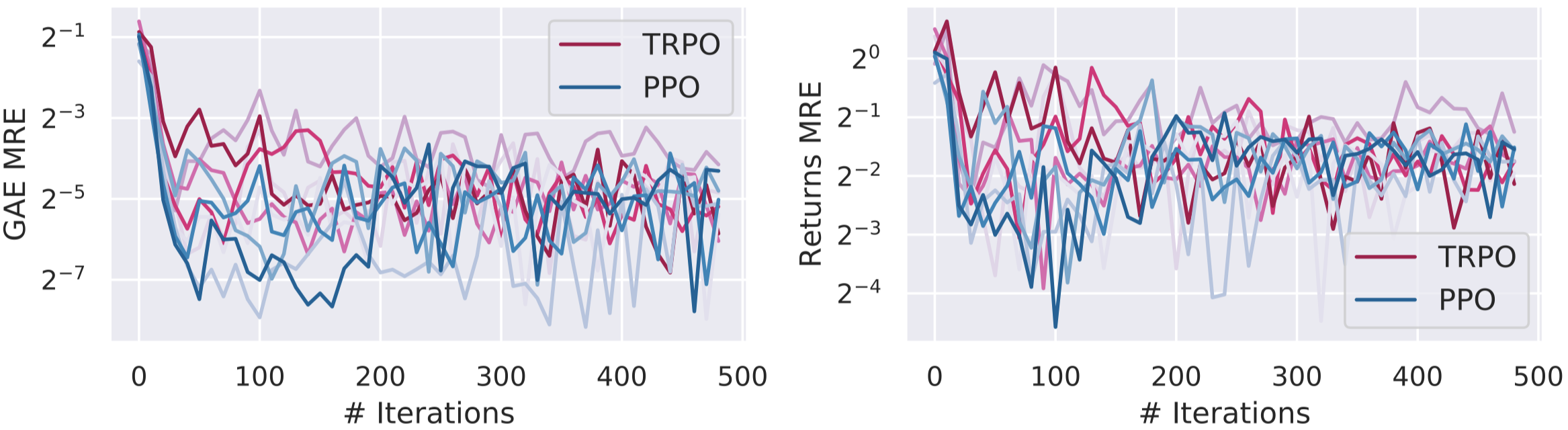
The above plots suggest that although the value network minimizes the GAE loss effectively, it likely does not predict the true value function. This discrepancy might perhaps challenge our conceptual understanding of the value networks and the role their play.
From a practical standpoint, however, the utility of the value network comes solely from one aspect: its being an effective baseline for gradient variance reduction. This leads us to our second question: How good is the learned value network at reducing the variance of our policy gradient estimates? In particular, how does this variance reduction compare to that offered by the optimal or true value function?
With this goal in mind, we design the following experiment. We first train an agent and freeze it at different iterations. For each of the resulting agents, we train a new value network using the true objective \eqref{eq:returnsloss}, and a very large number of trajectories (5 million state-action pairs). Since employing such a large training set lets us closely predict the true state values, we call the obtained value network the “true” value network.
We then examine how effectively this “true” value network reduces gradient variance - compared to the GAE-based value network and, as another baseline, a trivial constant “zero” value network. To measure gradient variance we complete similar experiments as earlier – for each agent and value network pair, we independently calculate gradient estimates and calculate their mean pairwise cosine similarity (and repeat this experiment while varying the number of samples used; note that we experiment in the Walker-2d environment here).
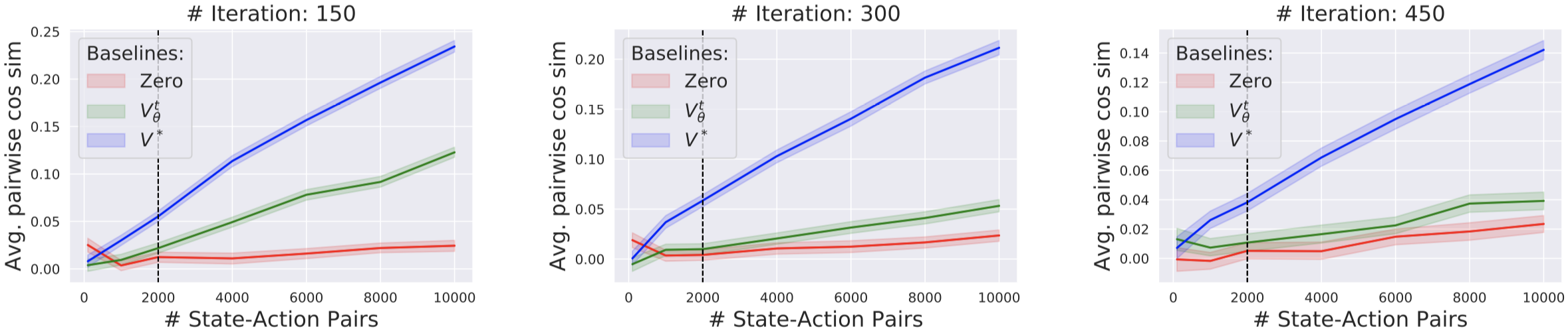
Our results indicate that the value network does reduce variance compared to the “zero” baseline. But there is still much room for improvement compared to what one can achieve using the “true” value function.
Now, it is important to keep in mind that, despite this relative improvement achieved by the GAE-based value network appearing small, it might actually make a big difference, given the high variance of the original estimate. Indeed, it turns out that the agents trained with the GAE-based value network often attain order of magnitude larger rewards than those trained with the “zero” baseline.
Also, even if the above findings might be illuminating, we still lack a crisp understanding of the role of the value network in training. For example, how does the loss function used to train the value network actually impact value prediction and variance reduction? Moreover, can we empirically quantify the relationship between variance reduction and performance? Finally, though we capture here the value network’s ability to reduce variance, it is unclear whether the network assumes a broader role in policy gradient methods.
In our next post, we’ll conclude our investigation of policy gradient methods (for now) by examining the reward landscape and the methods with which these algorithms explore it.