This post is the last of a three part series about our recent paper: “Are Deep Policy Gradient Algorithms Truly Policy Gradient Algorithms?” Today, we will analyze agents’ reward landscapes as well as try to understand to what extent, and by what mechanisms, our agents enforce so-called trust regions.
First, a quick recap (it’s been a while!):
-
In our first post, we outlined the RL framework and introduced policy gradient algorithms. We saw that auxiliary optimizations hidden in the implementation details of RL algorithms drastically impact performance. These findings highlighted the need for a more fine-grained analysis of how algorithms really operate.
-
In our second post, we zoomed in on two algorithms: trust region policy optimization (TRPO) and proximal policy optimization (PPO). Using these methods as a test-bed, we studied core primitives of the policy gradient framework: gradient estimation and value prediction.
Our discussion today begins where we left off in our second post. Recall that last time we studied the variance of the gradient estimates our algorithms use to maximize rewards. We found (among other things) that, despite high variance, algorithm steps were still (very slightly) correlated with the actual, “true” gradient of the reward. However, how good was this true gradient to begin with? After all, a fundamental assumption of the whole policy gradient framework is that our gradient steps actually point in a direction (in policy parameter space) that increases the reward. Is this indeed so in practice?
Optimization Landscapes
Recall from our first post that policy gradient methods treat reward maximization as a zeroth-order optimization problem. That is, they maximize the objective by applying first order methods with finite sample gradient estimates of the form:
\[\begin{align*} \nabla_\theta \mathbb{E}_{\tau \sim \pi_\theta} \left[r(\tau) \right] &= \mathbb{E}_{\tau \sim \pi_\theta} \left[g(\tau)\right] \\ &\approx \frac{1}{N} \sum_{\tau \sim \pi_\theta} \left[ g(\tau) \right] \end{align*}\]Here, \(r(\tau)\) represents the cumulative reward of a trajectory \(\tau\), where \(\tau\) is sampled from the distribution of trajectories induced by the current policy \(\pi_\theta\). We let \(g(\tau)\) represent an easily computable function of \(\tau\) that is an unbiased estimator of the gradient of the reward (seen on the left hand side)—for more details see our previous post. Finally, we denote by \(N\) the number of trajectories used to estimate the gradient.
An important point is, however, that instead of following the gradients of the cumulative reward (as suggested by the above equation), the algorithms we analyze actually use a surrogate reward at each step. The surrogate reward is a function of the collected trajectories that is meant to locally approximate the true reward, while providing other benefits such as easier computation and a smoother optimization landscape. Consequently, at each step these algorithms maximize the surrogate rewards \(r_{surr}(\tau)\) instead of following the gradient of the true reward \(r(\tau)\).
A natural question to ask is: do steps maximizing the surrogate reward consistently increase policy returns? To answer this, we will use landscape plots as a tool for visualizing the landscape of returns around a given policy \(\pi_\theta\):
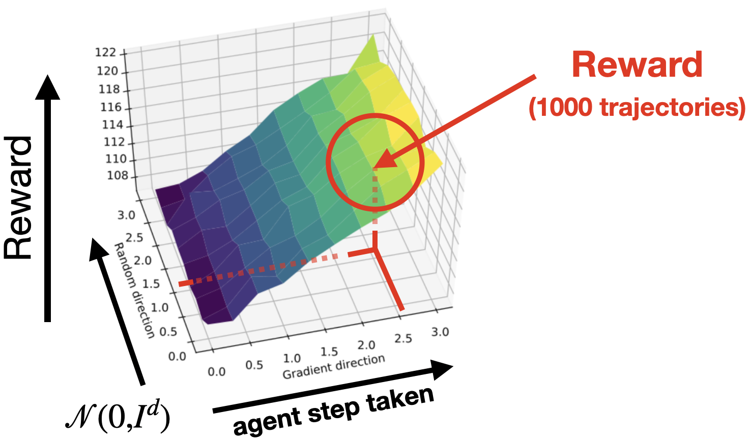
Here, for each point \((x, y, z)\) in the plot, \(x\) and \(y\) specify a policy \(\pi_{\theta’}\) parameterized by
\[\theta’ = \theta + x\cdot \widehat{g} + y \cdot\mathcal{N}(0,I),\]where \(\widehat{g}\) is the step computed by the studied algorithm. (Note that we include the random Gaussian \(\mathcal{N}(0,I)\) direction to visualize how “important” the step direction is compared to a random baseline). The \(z\) axis corresponds to the return attained by the policy \(\pi_{\theta’}\), which we denote by \(R(\theta’)\).
Now, when we make this plot for a random \(\theta\) (corresponding to a randomly initialized policy network), everything looks as expected:
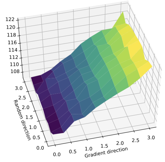
That is, the return increases significantly more quickly along the step direction than in the random direction. However, repeating these landscape experiments at later iterations, we find a more surprising picture: going in the step direction actually decreases the average cumulative reward obtained by the resulting agent!
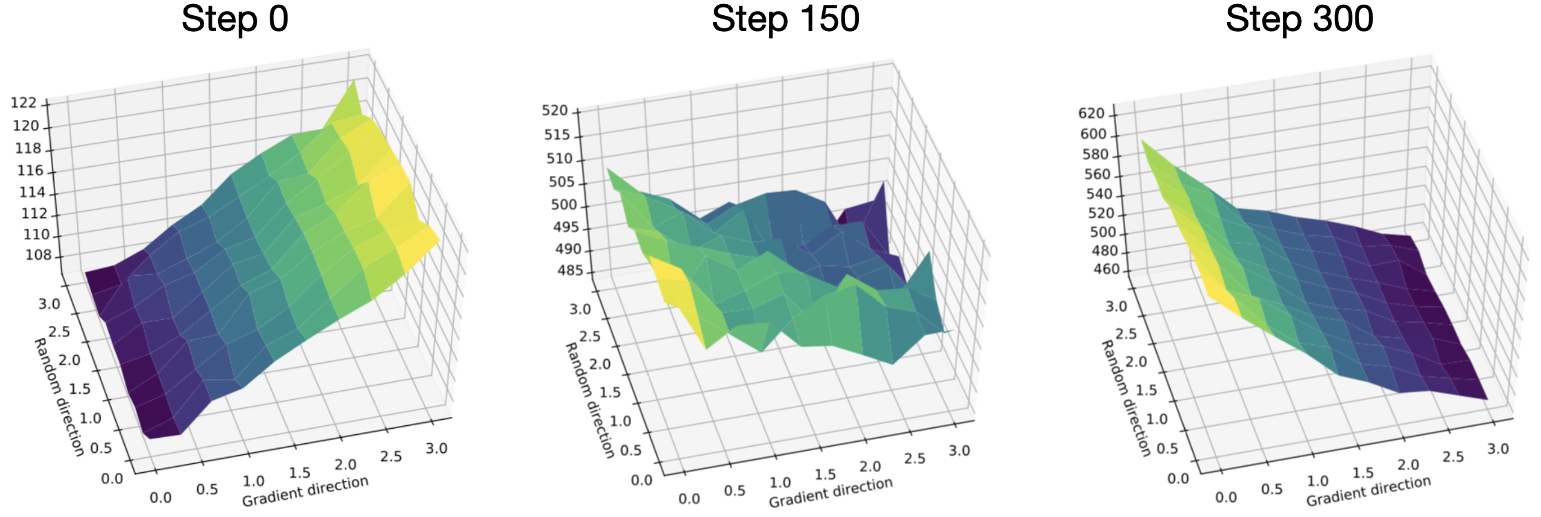
So what exactly is going on here? The steps computed by these algorithms are estimates of the gradient of the reward, so it is unexpected that the reward plateaus (or in some cases decreases!) along this direction.
We find that the answer lies in a misalignment of the true reward and the surrogate. Specifically, while the steps taken do correspond to an improvement in the surrogate problem, they do not always correspond to a similar improvement in the true return. Here are the same graphs as above shown again, this time with the corresponding optimization landscapes of the surrogate loss 1:
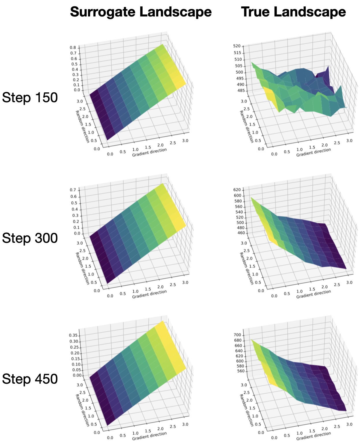
To make matters worse, we find that in the low sample regime that policy gradient methods actually operate in, it is hard to even discern directions of improvement in the true reward landscape. (In all the plots above, we use orders of magnitude more samples than an agent would ever see in practice at a single step.) In the plot below, we visualize reward landscapes while varying the number of samples used to estimate the expected return of a policy \(R(\theta’)\):
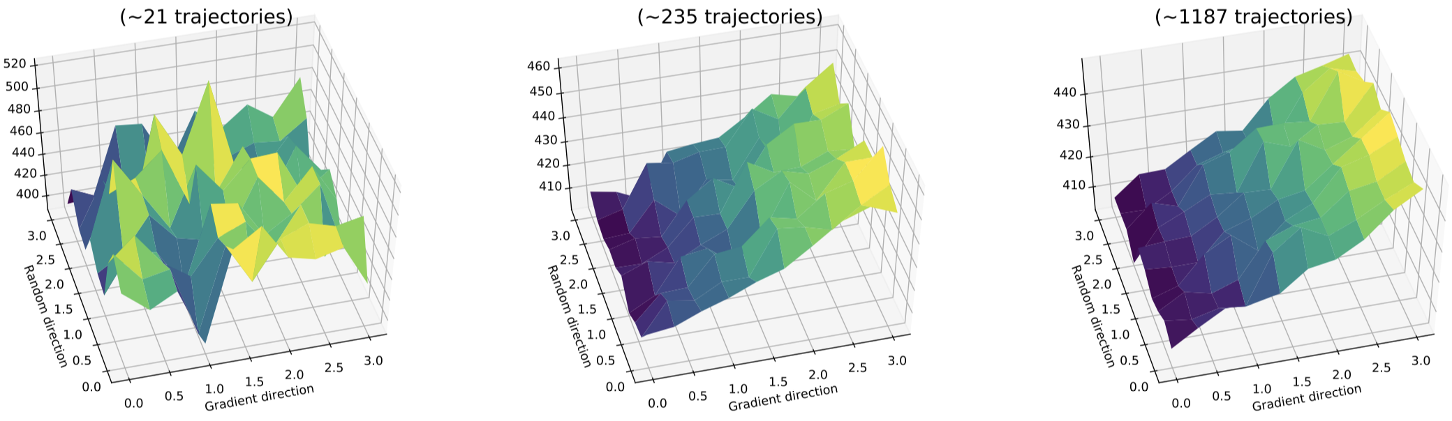
In contrast to the smooth landscape we see on the right and in the plots above, the reward landscape actually accessible to the model is jagged and poorly behaved. This landscape makes it thus near-impossible for an agent to distinguish between good and bad points in its relevant sample regime, even when the true underlying landscape is fairly well-behaved!
Overall, our investigation into the optimization landscape of policy gradient algorithms reveals that (a) the surrogate reward function is often misaligned with the underlying true return of the policy, and (b) in the relevant sample regime, it is hard to distinguish between “good” steps and “bad” steps, even when looking at the true reward landscape. As always, however, none of this stops the agents from training and continually improving reward in the average sense. This raises some key questions about the landscape of policy optimization:
- Given that the function we actually optimize is so often misaligned with the underlying rewards, how is it that agents continually improve?
- Can we explain or link the local behaviour we observe in the landscape with a more global view of policy optimization?
- How do we ensure that the reward landscape is navigable? And, more generally, what is the best way to navigate it?
Trust Regions
Let us now turn our attention to another important notion in the popular policy gradient algorithms: that of the trust region. Recall that a convenient way to think about our training process is to view it as a series of policy parameter iterates:
\[\theta_1 \to \theta_2 \to \theta_3 \to \cdots \rightarrow \theta_T\]An important aspect of this process is ensuring that the steps we take don’t lead us outside of the region (of parameter space) where the samples we collected are informative. Intuitively, if we collect samples at a given set of policy parameters \(\theta\), there is no reason to expect that these samples should tell us about the performance of a new set of parameters that is far away from \(\theta\).
Thus, in order to ensure that gradient steps are predictive, classical algorithms like the conservative policy update employ update schemes that constrain the probability distributions induced by successive policy parameters. The TRPO paper in particular showed that one can guarantee monotonic policy improvement with each step by solving a surrogate problem of the following form:
\[\begin{equation} \tag{1} \label{eq:klpen} \max_{\theta}\ R_{surr}(\theta) - C\cdot \left(\sup_{s} D_{K L}\left(\pi_{\theta}(\cdot | s) \| \pi_{\theta}(\cdot | s)\right)\right). \end{equation}\]The second, “penalty” term in the above objective, referred to as the trust region penalty, is a critical component of modern policy gradient algorithms. TRPO, one of the algorithms we study, proposes a relaxation of \eqref{eq:klpen} that instead imposes a hard constraint on the mean KL divergence2 (estimated using the empirical samples we obtain):
\[\begin{equation} \tag{2} \label{eq:trpotrust} \max_{\theta}\ R_{surr}(\theta) \qquad \text{such that} \qquad \mathbb{E} \left[ D_{KL} \left(\pi_{\theta}(\cdot | s) \| \pi_{\theta}(\cdot | s) \right) \right] \leq \delta. \end{equation}\]In other words, we try to ensure that the average distance between conditional probability distributions is small. Finally, PPO approximates the mean KL bound of TRPO by attempting to constrain a ratio between successive conditional probability distributions, instead of the KL divergence. The exact mechanism for enforcing this is shown in the box below. Intuitively, however, what PPO does is just throw away (i.e. get no gradient signal from) the rewards incurred from any state-action pair such that:
\[\begin{equation} \tag{3} \label{eq:ratio} \frac{\pi_{\theta_{t+1}}(a|s)}{\pi_{\theta_t}(a|s)} > 1 + \epsilon, \end{equation}\]where \(\epsilon\) is a user-chosen hyperparameter.
The exact update used by PPO is as follows, where $\widehat{A}_\pi$ is the generalized advantage estimate: $$ \begin{array}{c}{\max _{\theta} \mathbb{E}_{\left(s_{t}, a_{t}\right) \sim \pi}\left[\min \left(\operatorname{clip}\left(\rho_{t}, 1-\varepsilon, 1+\varepsilon\right) \widehat{A}_{\pi}\left(s_{t}, a_{t}\right), \rho_{t} \widehat{A}_{\pi}\left(s_{t}, a_{t}\right)\right)\right]} \\ {\text{where }\ \ \rho_{t}=\frac{\pi_{\theta}\left(a_{t} | s_{t}\right)}{\pi\left(a_{t} | s_{t}\right)}}\end{array} $$ As described in the main text, this intuitively corresponds to throwing away (i.e. getting no gradient signal) from state-action pairs where the ratio of conditional probabilities between successive policies is too high.
To recap, there is a theoretically motivated algorithm \eqref{eq:klpen} which constrains maximum KL. This motivates TRPO’s bound on mean KL in \eqref{eq:trpotrust}, which in turn motivates the ratio-based bound of PPO (shown in the box). This chain of approximations might lead us to ask: how well do these algorithms actually maintain trust regions?
We first plot the mean KL divergence between successive policies for each
algorithm:
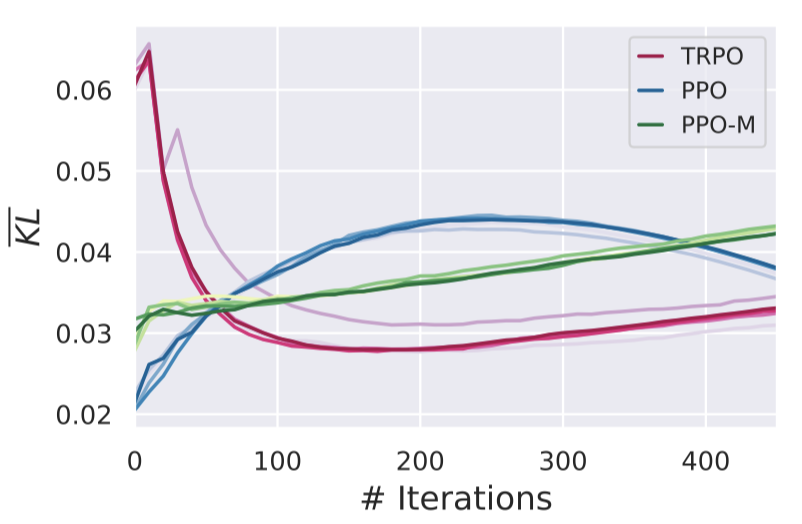
TRPO seems to constrain this very well 3 ! On the other hand, our two varieties of the PPO algorithm paint a drastically different picture. Recall that we decided to separately study two versions of PPO: PPO (based on a state-of-the-art implementation), and PPO-M, which we defined to be the core PPO algorithm without auxiliary optimizations (PPO-M is the core PPO algorithm exactly as described in the original paper, without any of the auxiliary optimizations). Both PPO with optimizations and PPO-M do quite well at maintaining a KL trust region. However, their mean KL curves are rather different due to auxiliary optimizations such as Adam learning rate annealing or orthogonal initialization.
Despite seeming to enforce a mean KL trust region, it turns out that PPO does not successfully enforce its own ratio-based trust region. Below, we plot the maximum ratio \eqref{eq:ratio} between successive policies for the three algorithms in question:
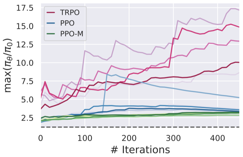
In the above, the dotted line represents \(1+\epsilon\), corresponding to the bound in \eqref{eq:ratio}—it looks like the max ratio is not kept at all! And once again, simply adding the auxiliary, code-level optimizations to PPO-M yields better trust region enforcement, despite the main clipping mechanism staying the same. Indeed, it turns out that the way that PPO enforces the ratio trust region does not actually keep the ratios from becoming too large or too small. In fact, in our paper we show that there are infinite optima of the optimization problem PPO solves to find each step and only one of them enforces the intended trust region bound.
Wrapping Up
Deep reinforcement learning algorithms are rooted in a well-grounded framework of classical RL, and have shown great promise in practice. However, as we’ve found in our three-part investigation, this framework often falls a little short of explaining the behavior of these algorithms in practice.
Beyond just being disconcerting, this disconnect impedes our understanding of why these algorithms succeed (or fail). It also poses a major barrier to addressing key challenges facing deep RL, such as widespread brittleness and poor reproducibility (as has been observed by our study in part one and many others, e.g., [1, 2, 3]).
To close this gap, we need to either develop methods that adhere more closely to theory, or build theory that can capture what makes existing policy gradient methods successful. In both cases, the first step is to precisely pinpoint where theory and practice diverge. Even more broadly, our findings suggest that developing a deep RL toolkit that is truly robust and reliable will require moving beyond the current benchmark-driven evaluation model, to a more fine-grained understanding of deep RL algorithms.