Generative AI models are impressive. Yet, how exactly do they use the enormous amounts of data they are trained on? In our latest paper, we take a step towards answering this question through the lens of data attribution.
In the last year, the tech world has been taken over by generative AI—models (such as ChatGPT and Stable Diffusion). The key driver for the impressive performance of these models is the large amount of data used to train them. Yet, we still lack a good understanding of how exactly this data drives their performance. An understanding that could be especially important in light of recent concerns that they might be copying their training data.
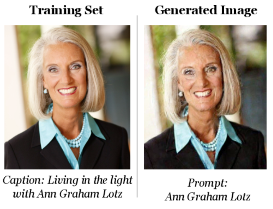
Indeed, as previous work suggested, in some cases, generative models might be copying from their training data when synthesizing new images. This is pretty clear in the example below from this paper: the image on the left below is an image from Wikipedia, while the image on the right was generated by Stable Diffusion and they look almost identical!
In most cases, however, it is not as obvious what training images the model is using when generating a new sample. For instance, the model might be combining small parts of many images to generate this new sample. It would thus be useful to have a more principled way to answer the question, “which training examples caused my model to do X?” (in our case, X is “generate this image”).
This is exactly the problem of data attribution, which has been well studied in the machine learning literature, including some of our own work. However, almost all this work has focused on the supervised setting. It turns out that extending data attribution to generative models poses new challenges.
First of all, it is not obvious what we want to be attributing. For example, given an image generated by a diffusion model, some training examples might be responsible for the background, while others might be responsible for the foreground. Do we have a preference here? Second, we need to work out a way to verify attributions. That is, how can we be sure that the training images identified by an attribution method are indeed responsible for generating a given image?
We address exactly these challenges in our latest paper. Let’s dive in!
Diffusion Process: A Distributional View
Diffusion models generate images via a multi-step process: the model begins with random noise, and gradually de-noises the intermediate latents (i.e., noisy images) over many steps to arrive at a final generated image (see these blogs for a more in-depth description). How can we study this complex process and attribute it back to the training data?
Let’s first take a look at this process from a different angle: instead of looking at just the sampled trajectory, consider the entire distribution of images that we can sample starting from a given intermediate step $t$. Here is what we get when we consider this question for different steps $t$:
Notice that at first, this distribution seems to cover a wide range of possible final images (since the model hasn’t “decided” on much yet). However, towards later steps this process gradually “narrows down” to the final generated image. So, studying how this distribution evolves over steps can give us a natural way to identify the impact of each step of a given image generation.
One Step at a Time: Attributing the Diffusion Process
Motivated by the above observation, we attribute how training data affects each step of the generation process: the goal is to quantify the impact of each training example on the distribution of images generated by the model conditioned on the intermediate latent at each step $t$. So, intuitively, a training example is positively (negatively) influential at time $t$ if it increases (decreases) the likelihood that the final image is generated starting from step $t$.
Now that we have established what we want to attribute, we can efficiently compute these attributions by adapting TRAK, our recent work for data attribution in the supervised setting that builds on the datamodeling framework. Formalizing attribution in this way allows us to come up with natural ways to evaluate them too.
We leave the details of the method and evaluation to our paper—and now let’s just visualize what the resulting attributions look like!
Let’s start with a simple example in which we trained a diffusion model on the CIFAR-10 dataset:
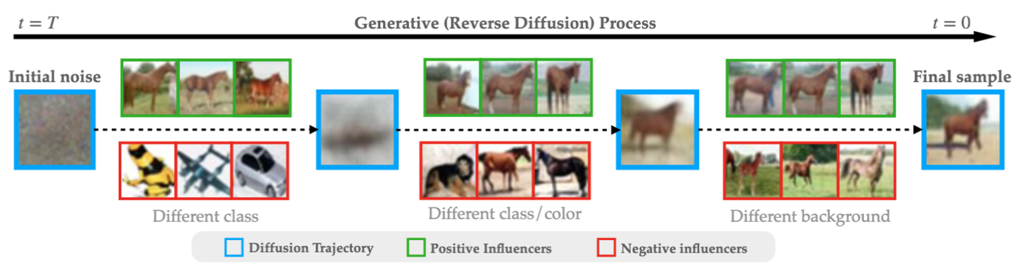
Here, we present the images from the training set that have the strongest (positive or negative) influence on the diffusion model (according to our method) when it’s synthesizing the above image of a horse. Again, the positive influencers are the images that steer the model towards the final generated image. Conversely, the negative influencers steer the model away from it.
And here is what happens in a bit more advanced case. That is, when we repeat the same procedure for text-guided latent diffusion models trained on the MS-COCO dataset, after using the prompt “three flower with vases”:
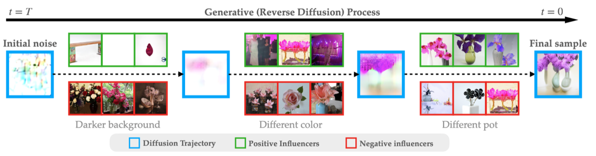
Note that the same image (three pink flowers on yellow background) is one of the most positive influencers at some point, but later on is one of the most negative ones!
And here are some more examples, presented more compactly as animations:
 |
 |
 |
 |
 |
 |
Isolating Image Features with Diffusion Steps
It turns out that attributing at individual steps unlocks yet another benefit: the ability to surface attributions for individual features in a generated image. Specifically, let’s look again at the distribution of images arising from conditioning the diffusion model on the intermediate latent at each step $t$. This time, we’ll also plot the fraction of samples at each step that contain a particular feature (in this case, the feature is whether the image contains a horse):
On the left side, we plot the fraction of images in that distribution that contain a horse (according to a pre-trained classifier). Curiously, notice the “sharp transition” around step 600: in just a very narrow interval of steps, the diffusion model decides that the final image will contain a horse!
We find that these kinds of sharp transitions occur often (we give more examples in our paper). And this, in turn, enables us to attribute features of the final image to training examples. All we need to do is to find attributions for the interval of steps where the likelihood of a given feature has the sharpest increase. So, in our example above, to attribute the presence of a horse in the above image, we can focus our attributions to around step 600.
It turns out that our attributions line up incredibly well with the evolution of features. For instance, in the right side of the figure above, we show the top influencers (in green) and bottom influencers (in red) at each step. Notice that before the likelihood begins to increase, none of the influencers contain horses. But, after the likelihood reaches 100%, suddenly both the positive and negative influencers are horses! However, around step 600, the positive influencers contain horses while the negative influencers don’t—this is precisely the step at which the likelihood of the original model generating a horse rapidly changes.
In our paper, we show that this “sharp transition behavior” holds in more complex settings, such as Stable Diffusion models trained on LAION, too.
Bonus Snippet: Attributing Patches
Sometimes, isolating individual steps might not enough to disentangle a feature of interest. For example, in the image below, the motorcycle and stop sign might be decided in an overlapping set of steps. In this case, we can however introduce a modification to our data attribution method to attribute patches within an image that correspond to features. As we show below, this modification allows us to directly identify training images that are influential to parts of the generated images.
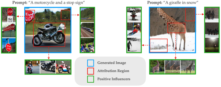
For example, notice that when we focus on the patch corresponding to the motorcycle, we identify training examples that contain motorcycles. However, when we focus on the patch corresponding to the background, we identify training examples that contain similar backgrounds.
Conclusion
In this post, we studied the problem of data attribution for diffusion models as a step towards understanding how these models use their training data. We saw how it’s useful to consider the distribution of possible final samples throughout the steps of the diffusion process to see how the model “narrows down” to the final generated image, and to attribute each step of this process individually. We then visualized the resulting attributions, and found that they are both visually interpretable and can help us to isolate the training images most responsible for particular features in a generated image. In our paper, we give more details about how we implement our method, and we also extensively evaluate our attributions to verify their counterfactual significance.
Overall, our approach shows that it’s possible to meaningfully attribute generative outputs from even complex models like modern diffusion pipelines back to training data.